Recurrent neural networks (RNNs) are a family of neural networks for processing sequential data. RNNs are generally used to implement language models. We, as humans, base much of our language understanding on the context. For example, let's consider the sentence Christmas falls in the month of --------. It is easy to fill in the blank with the word December. The essential idea here is that there is information about the last word encoded in the previous elements of the sentence.

The central theme behind the RNN architecture is to exploit the sequential structure of the data. As the name suggests, RNNs operate in a recurrent way. Essentially, this means that the same operation is performed for every element of a sequence or sentence, with its output depending on the current input and the previous operations.

An RNN works by looping an output of the network at time t with the input of the network at time t+1. These loops allow persistence of information from one time step to the next one. The following diagram is a circuit diagram representing an RNN:

The diagram indicates an RNN that remembers what it knows from previous input using a simple loop. This loop takes the information from the previous timestamp and adds it to the input of the current timestamp. At a particular time step t, X_t is the input to the network, O_t is the output of the network, and h_t is the detail it remembered from previous nodes in the network. In between, there is the RNN cell, which contains neural networks just like a feedforward network.

Let's consider an example sentence: Christmas Holidays are Awesome. In this sentence, take a look at the following timestamp:

• Christmas is x₀
• Holidays is x₁
• are is x₂;
• Awesome is x₃

If t=1, then take a look at the following:

• x_t = Holidays → event at current timestamp
• x_t-1 = Christmas → event at previous timestamp

It can be observed from the preceding circuit diagram that the same operation is performed in the RNN repeatedly on different nodes. There is also a black square in the diagram that represents a time delay of a single time step. It may be confusing to understand the RNN with the loops, so let's unfold the computational graph. The unfolded RNN computational graph is shown in the following diagram:

In the preceding diagram, each node is associated with a particular time. In the RNN architecture, each node receives different inputs at each time step x_t. It also has the capability of producing outputs at each time step o_t. The network also maintains a memory state h_t, which contains information about what happened in the network up to the time t. As this is the same process that is run across all the nodes in the network, it is possible to represent the whole network in a simplified form, as shown in the RNN circuit diagram.

Now, we understand that we see the word recurrent in RNNs because it performs the same task for every element of a sequence, with the output depending on previous computations. It may be noted that, theoretically, RNNs can make use of information in arbitrarily long sequences, but in practice, they are implemented to looking back only a few steps.

Formally, an RNN can be defined in an equation as follows:

In the equation, h_t is the hidden state at timestamp t. An activation function such as Tanh, Sigmoid, or ReLU can be applied to compute the hidden state and it is represented in the equation as . W is the weight matrix for the input to the hidden layer at timestamp t. X_t is the input at timestamp t. U is the weight matrix for the hidden layer at time t-1 to the hidden layer at time t, and h_t-1 is the hidden state at timestamp t.

During backpropagation, U and W weights are learned by the RNN. At each node, the contribution of the hidden state and the contribution of the current input are decided by U and W. The proportions of U and W in turn result in the generation of output at the current node. The activation functions add non-linearity in RNNs, thus enabling the simplification of gradient calculations during the backpropagation process. The following diagram illustrates the idea of backpropagation:

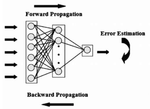
The following diagram depicts the overall working mechanism of an RNN and the way the weights U and W are learned through backpropagation. It also depicts the use of the U and W weight matrices in the network to generate the output, as shown in the following diagram: