
8
Vibrations of Spring–Mass Systems and Thin Beams
8.1 Introduction
The time-varying response and the frequency response of single and two degrees-of-freedom systems for various loadings, initial conditions, and nonlinearities are examined by creating suitable interactive environments to explore their characteristics as a function of the parameters that govern the respective systems. Then, the determination of the natural frequencies and mode shapes for thin beams subject to various boundary conditions and loadings are examined. The following applications will be considered:
Single degree-of-freedom systems –
- effects of spectral content of periodic forces on the time-varying response;
- effects of squeeze film damping and viscous fluid damping on the amplitude response and phase response;
- stability in the presence of an electrostatic force;
- parameters that maximize the average power of a piezoelectric energy harvester.
Two degrees-of-freedom systems –
- effects of systems parameters on the amplitude response functions;
- system parameters that produce an enhanced piezoelectric energy harvester.
Thin beams –
- effects of in-span attachments on the natural frequencies and modes shapes of thin cantilever beams;
- effects of an electrostatic force on the lowest natural frequency and the stability of beams;
- effects of in-span attachments on the response of a cantilever beam to an impulse force.
For each of these topics, we shall use Manipulate to create an interactive graphic to explore the system response to the variation of its parameters.
8.2 Single Degree-of-Freedom Systems
8.2.1 Periodic Force on a Single Degree-of-Freedom System
Consider a single degree-of-freedom system with a mass m (kg), a spring of stiffness k (N·m−1), and a viscous damper with damping coefficient c (N·s·m−1). The mass is subjected to periodic force of magnitude Fo (N) and period T = 2π/ωo (s), where ωo (rad·s−1) is the fundamental frequency of the forcing. If the periodic force is expressed as a Fourier series, then the displacement response of the mass is [1, p. 259–264]

where Ω0 = ωo/ωn, Ωl = lΩ0,

and
Two types of periodic pulses are considered; a single pulse and a double pulse, which are shown in Figure 8.1. For the single pulse of duration τd, the coefficients are
and, therefore,
where α = Ω0τd/2π. For the double pulse that is positive for 0 ≤ τ ≤ τd and negative for τd ≤ τ ≤ 2τd, the coefficients are


Figure 8.1 Initial configuration of the interactive graph to explore the response of a single degree-of-freedom system to two different periodic waveforms
An interactive figure shown in Figure 8.1 shall be created so that one can explore how the spectral content of the periodic force affects the time domain waveform as a function of α, Ωo, and ζ. The time-domain signal is given by Eq. (8.1), where the spectral content before being applied to the system is given by cl and that of the mass is given by clH(Ωl). We shall use 150 terms in the Fourier series expansion. The program that creates Figure 8.1 is as follows.
Manipulate[
(* Evaluate Eq. (8.2) *)
   hh=1/Sqrt[(1-(r Ω0)^2)^2+(2 ζ r Ω0)^2];
   thh=ArcTan[1-(r Ω0)^2,2 ζ r Ω0];
(* Obtain coefficients from either Eq. (8.5) or Eq. (8.6) *)
   cnn=If[ptyp==1,Abs[Sin[r π α]/(r π α)],
      a1=(2 Sin[2 π α r]-Sin[4 π α r])/(π r);
      b1=(1-2 Cos[2 π α r]+Cos[4 π α r])/(π r);
      Sqrt[a1^2+b1^2]];
   psnn=If[ptyp==1,ArcTan[1-Cos[2 r π α],Sin[2 r π α]],
      ArcTan[b1,a1]];
   ptin=Table[{n,cnn[[n]]},{n,1,nn}];
   ptout=Table[{n,hh[[n]] cnn[[n]]},{n,1,nn}];
   lines=Table[{{n,0},{n,If[cnn[[n]]<hh[[n]] cnn[[n]],
      hh[[n]] cnn[[n]],cnn[[n]]]}},{n,1,nn}];
(* Sum series: Eq. (8.1) *)
   xt=If[ptyp==1,α+2 α Total[cnn hh Sin[r Ω0 t-thh+psnn]],
      Total[cnn hh Sin[r Ω0 t-thh+psnn]]];
(* Coordinates to draw pulse *)
   If[ptyp==1,
      pulse1={{0,0},{0,1},{2 π α/Ω0,1},{2 π α/Ω0,0}};
      pulse2={{2 π/Ω0,0},{2 π/Ω0,1}, {π α/Ω0+2 π/Ω0,1}},
      pulse1={{0,0},{0,1},{2 π α/Ω0,1},{2 π α/Ω0,-1},
         {4 π α/Ω0,-1},{4 π α/Ω0,0}};
      pulse2={{2 π/Ω0,0},{2 π/Ω0,1}, {2 π α/Ω0+2 π/Ω0,1}}];
(* Create two graphs, one above the other *)
   GraphicsColumn[{Plot[xt,{t,-π/Ω0/5.,
      2 π/Ω0+π α/Ω0},PlotStyle->{Red},
      PlotRange->{Full,{-2,2.3}},PlotLabel->label1,
      AxesLabel->{"τ","Amplitude"},
      Epilog->{{Blue,Line[pulse1]},{Blue,Line[pulse2]}}],
      ListLinePlot[lines,PlotStyle->Black,
         PlotRange->{{0,nn+1},Full},PlotLabel->label2,
         AxesLabel->{"n=Ωn/Ω0","Magnitude"},
         Epilog->{{Blue,PointSize[Medium],Point[ptin]},
         {Red,PointSize[Medium],Point[ptout]}}]}],
(* Create sliders and radio buttons *)
   Style["Periodic Waveform",Bold],
   {{ptyp,1," "},{1->labs,2->labd}, ControlType->RadioButton},
   Delimiter,
   Style["Input Parameters",Bold],
   {{Ω0,0.04,"Ωo"},0.01,1,0.01,Appearance->"Labeled",
      ControlType->Slider},
   {{α,0.2,la},0.02,0.49,0.01,Appearance->"Labeled",
      ControlType->Slider},
   Delimiter,
   Style["Damping Factor",Bold],
   {{ζ,0.1,"ζ"},0.02,0.7,0.01,Appearance->"Labeled",
      ControlType->Slider},
   Delimiter,
   Style["Frequency Spectrum -",Bold],
   Style[" Maximum Number of Harmonics Displayed",Bold],
   {{nn,20,"N"},1,50,1,Appearance->"Labeled",
      ControlType->Slider},
   ControlPlacement->Left,
   Initialization:>(puls={{0,0},{0,1},{0.25,1},{0.25,0},
      {1,0},{1,1},{1.1,1}};
(* Radio button images *)
   labs=ListLinePlot[puls,PlotRange->{{0,1.2},{-0.1,1}},
      Axes->False,ImageSize->Tiny,Epilog->{Arrowheads[0.1],
         Arrow[{{0,0.5},{1,0.5}}],Arrow[{{1,0.5},{0,0.5}}],
         Inset[Style["2π/Ω0",14],{0.5,0.65}],
         Inset[Style["τd",14],{0.125,0.1}]}];
   puld={{0,0},{0,1},{0.15,1},{0.15,-1},{0.3,-1},{0.3,0},
      {1,0},{1,1},{1.1,1}};
   labd=ListLinePlot[puld,PlotRange->{{0,1.2},{-1.1,1}},
      Axes->False,ImageSize->Tiny,
      Epilog->{Arrowheads[{-0.1,0.1}],
         Arrow[{{0,0.5},{1,0.5}}],
         Inset[Style["2π/Ω0",14],{0.5,0.75}],
         Inset[Style["τd",14],{0.075,0}]}];
(* Figure titles *)
   label1=Column[{"Time Domain Waveforms",
      Row[{Style["Input, ",Blue],
      Style["Output ",Red]}]},Center];
    label2=Column[{"Frequency (Harmonic) Spectrum",
      Row[{Style[Row[{"Input cn"}],Blue],
      Style[Row[{" Output [cnH(Ωn)]"}],Red]}]},Center];
(* Slider label *)
   la="α=Ωoτd/(2π)"; r=Range[1,150];),
   TrackedSymbols:>{Ω0,α,ζ,nn,ptyp}]
8.2.2 Squeeze Film Damping and Viscous Fluid Damping
We shall examine the amplitude response and phase response of a single degree-of-freedom system undergoing harmonic oscillations at frequency ω when the system is subjected to squeeze film damping and viscous fluid damping. The single degree-of-freedom system has a mass m (kg) and a spring of stiffness k (N·m−1).
Squeeze Film Damping
Squeeze film air damping is caused by the entrapment of air between two parallel surfaces that are moving relative to each other in the normal direction. For this damping, the amplitude response and phase response, respectively, for a base-excited spring–mass system when the surface of the mass that is in contact with an air film has a rectangular shape are [2, Section 2.3]
where

and

The quantity σn is the squeeze number at ωn, where ωn is defined in Eq. (8.3). In Eq. (8.8), β = a/L is the aspect ratio of the rectangular shape such that for a narrow strip, β → ∞ and for a square surface β = 1. The film depth is ho, μ is the dynamic viscosity (N·s·m−2) of the gas between the two surfaces, A is the area of the surfaces, and Pa is the atmospheric pressure in the gap ho.
Viscous Fluid Damping
Approximations of viscous fluid damping are obtained by considering the mass to be a long rigid circular cylinder of length L, density ρm, and diameter b that is oscillating harmonically at a frequency ω in a fluid of infinite extent and density ρf. The response functions for a mass-excited system with viscous fluid damping are [2, Section 2.4]

where
and

In Eq. (8.10), Kn(x) is the modified Bessel function of the second kind of order n, Ren is the Reynolds number at frequency ωn, and μf is the dynamic viscosity (N·s·m−2). The quantity Γ is called the hydrodynamic function, and it is noted that Imag[Γ] is negative so that ce is positive.
We shall create an interactive figure shown in Figure 8.2 from which one can explore the effects that the two types of damping have on the amplitude response and phase response of a single degree-of-freedom system and for each type of damping show how the corresponding damping parameters affect these responses. In Eq. (8.8), the maximum values of l and m are 51. The program that creates Figure 8.2 is as follows.

Figure 8.2 Initial configuration of the interactive graph to determine the amplitude response and phase response of a single degree-of-freedom system for two types of damping
Manipulate[
(* Select appropriate amplitude response function: Eq. (8.7) or Eq. (8.9) *)
   ampl=Which[funk==1,1/Sqrt[(1+rk srk[σ,Ω,β]-Ω^2)^2+
      (rk srd[σ,Ω,β])^2],
      funk==2,gc=1+4 BesselK[1,Sqrt[I ren Ω]]/
      (Sqrt[I ren Ω] BesselK[0,Sqrt[I ren Ω]]);
      1/Sqrt[(1-(1+rfrm Re[gc]) Ω^2)^2+(-rfrm Ω^2 Im[gc])^2]];
(* Select appropriate phase response function: Eq. (8.7) or Eq. (8.9) *)
phase=Which[funk==1,
   ArcTan[1+rk srk[σ,Ω,β]-Ω^2,rk srd[σ,Ω,β]]/Degree,
      funk==2,
      gc=1+4 BesselK[1,Sqrt[I ren Ω]]/(Sqrt[I ren Ω]*
         BesselK[0,Sqrt[I ren Ω]]);
      ArcTan[1-(1+rfrm Re[gc]) Ω^2,-rfrm Ω^2 Im[gc]]/Degree];
(* Create two graphs, one above the other *)
   GraphicsColumn[{Plot[ampl,{Ω,0,2},
      PlotRange->{{0,2},All},AxesLabel->{"Ω","Amplitude"},
      Epilog->{Red,Dashed,Line[{{1,0},{1,500}}]}],
   Plot[phase,{Ω,0,2},PlotRange->{{0,2},{0,180}},
      AxesLabel->{"Ω","Phase (°)])"},Epilog->{Red,Dashed,
         Line[{{{1,0},{1,180}},{{0,90},{2,90}}}]}]}],
(* Create sliders and popup menu *)
   Style["Damping Type",Bold],
   {{funk,2,""},{1->"Squeeze film",2->"Viscous fluid"},
      ControlType->RadioButton},
   Delimiter,
   Style["Squeeze Film Damping: Rectangular Shape",Bold],
   {{σ,1,"σn"},0.5,200,0.5,Appearance->"Labeled",
      Enabled->If[funk==1,True,False],ControlType->Slider,
      ContinuousAction->False},
   {{β,1,"β"},1,10,1,Appearance->"Labeled",
      ControlType->Slider,Enabled->If[funk==1,True,False],
      ContinuousAction->False},
   {{rk,1,Style["rk ",Italic]},0.5,2,0.05,
      Appearance->"Labeled",ContinuousAction->False,
      Enabled->If[funk==1,True,False],ControlType->Slider},
   Delimiter,
   Style["Viscous Fluid Damping",Bold],
   {{ren,200,"Ren"},0.1,1000,Appearance->"Labeled",
      Enabled->If[funk==2,True,False],ControlType->Slider,
      ContinuousAction->False},
   {{rfrm,0.9,"ρf/ρm"},0.05,1,0.05,Appearance->"Labeled",
      ControlType->Slider,ContinuousAction->False,
      Enabled->If[funk==2,True,False]},
   TrackedSymbols:>{σ,rk,ren,rfrm,funk,β},
(* Function representing Eq. (8.8) *)
   Initialization:>(
      srk[σ_,Ω_,β_]:=64. (Ω σ)^2/π^8 Total[Table[Total[Table[
         1/(m^2 n^2 (m^2+(n/β)^2)^2+(σ Ω)^2/π^4),
         {m,1,51,2}]],{n,1,51,2}]];
      srd[σ_,Ω_,β_]:=64. (σ Ω)/π^6*
         Total[Table[Total[Table[(m^2+(n/β)^2)/
            (m^2 n^2 ((m^2+(n/β)^2)^2+(σ Ω)^2/π^4)),
            {m,1,51,2}]],{n,1,51,2}]])]
8.2.3 Electrostatic Attraction
Consider a single degree-of-freedom system whose mass m (kg) is suspended by a spring with spring constant k (N·m−1) and a viscous damper with damping coefficient c (N·s·m−1). The bottom surface of the mass is rectangular with area A and is flat and parallel to a stationary flat surface. The distance between the two surfaces is do and there is a time varying voltage Vov(τ) that creates an electrostatic force, where v(τ) is the time-varying shape of the voltage of magnitude Vo (V). If the displacement of the mass is x and fringe correction factors are neglected, then the nondimensional form of the governing equation for this single degree-of-freedom system is given by [2, Section 2.5.2]

where τ and ζ are given in Eq. (8.3), w = x/do, and
The quantity ![]() o is the permittivity of free space, which for air is 8.854 × 10⁻¹² F·m−1. Equation (8.12) must be solved numerically.
o is the permittivity of free space, which for air is 8.854 × 10⁻¹² F·m−1. Equation (8.12) must be solved numerically.
For a given v(τ) and ζ, the solution to Eq. (8.12) is only stable when ![]() < (
< (![]() )max . At this value of (
)max . At this value of (![]() )max , w is denoted wmax. This quantity is determined interactively from the numerical evaluation of Eq. (8.12). The static displacement of the spring–mass system due to the electrostatic force is determined from
)max , w is denoted wmax. This quantity is determined interactively from the numerical evaluation of Eq. (8.12). The static displacement of the spring–mass system due to the electrostatic force is determined from
We shall create the interactive environment shown in Figure 8.3 from which one can obtain wmax from the displacement response as a function of ζ and ![]() when v(τ) = u(τ), where u(τ) is the unit step function. The interactive determination of the values of wmax and (
when v(τ) = u(τ), where u(τ) is the unit step function. The interactive determination of the values of wmax and (![]() )max , is facilitated by incrementing
)max , is facilitated by incrementing ![]() in steps of 0.0001. Hence, the slider is displayed with the optional controls visible, thus enabling one to have more precise control over this parameter’s values. In addition, because of the sensitivity of the solution method in the vicinity of (
in steps of 0.0001. Hence, the slider is displayed with the optional controls visible, thus enabling one to have more precise control over this parameter’s values. In addition, because of the sensitivity of the solution method in the vicinity of (![]() )max , the working precision of the numerical solution function is increased to 25. Also, the placement of the labels for wmax and wstatic is a function of tend. The program that creates Figure 8.3 is as follows.
)max , the working precision of the numerical solution function is increased to 25. Also, the placement of the labels for wmax and wstatic is a function of tend. The program that creates Figure 8.3 is as follows.

Figure 8.3 Initial configuration of the interactive graph to determine the displacement response of a single degree-of-freedom system to a suddenly applied electrostatic force
Manipulate[
(* Determine wstatic from Eq. (8.13) *)
fg=Min[x/.NSolve[x^3-2 x^2+x-eV==0,x]];
(* Solve Eq. (8.12) in terms of (eoVo)2 *)
   sol=Quiet[ParametricNDSolveValue[{w’’[t]+
      2 ζ1 w’[t]+w[t]==eVV/(1-w[t])^2,w[0]==w’[0]==0},
      w,{t,0,tend},{eVV,ζ1},WorkingPrecision->25]];
(* Determine maximum amplitude of solution to Eq. (8.12) *)
   bb=Quiet[NMaxValue[{sol[eV,ζ][t],2<t<18},t,
      WorkingPrecision->25]];
(* Plot results *)
   Plot[sol[eV,ζ][t],{t,0,tend},LabelStyle->{14},
      PlotRange->{{0,tend},{0,0.6}},
      AxesLabel->{τ,TraditionalForm[w[τ]]},
      Epilog->{{Red,Dashed,Line[{{0,fg},{tend,fg}}]},
         {Red,Dashed,Line[{{0,bb},{tend,bb}}]},
         Inset[Style[Row[{"wmax=",NumberForm[bb,4]}],
            Red,14],{0.8 tend,bb+0.025}],
         Inset[Style[Row[{"wstatic=",NumberForm[fg,4]}],
            Red,14],{0.8 tend,fg-0.03}]}],
(* Create sliders *)
Style["Applied Voltage Parameter",Bold],
{{eV,0.1329," "},0.12,0.1387,0.0001,
Appearance->{"Labeled","Open"}, ContinuousAction->False},
Delimiter,
Style["Damping Factor",Bold],
{{ζ,0.08,"ζ"},0.02,0.15,0.01,Appearance->"Labeled",
ContinuousAction->False,ControlType->Slider},
Delimiter,
Style["Axis Adjustment",Bold],
{{tend, 45,"τend"},35,200,5, Appearance->"Labeled",
ContinuousAction->False, ControlType->Slider},
TrackedSymbols:>{eV,ζ,tend}]
"},0.12,0.1387,0.0001,
Appearance->{"Labeled","Open"}, ContinuousAction->False},
Delimiter,
Style["Damping Factor",Bold],
{{ζ,0.08,"ζ"},0.02,0.15,0.01,Appearance->"Labeled",
ContinuousAction->False,ControlType->Slider},
Delimiter,
Style["Axis Adjustment",Bold],
{{tend, 45,"τend"},35,200,5, Appearance->"Labeled",
ContinuousAction->False, ControlType->Slider},
TrackedSymbols:>{eV,ζ,tend}]
Referring to Figure 8.3, the initial parameters were chosen such that if the + button on the animator/slider is depressed once; that is, ![]() is increased to 0.1330, the system becomes unstable.
is increased to 0.1330, the system becomes unstable.
8.2.4 Single Degree-of-Freedom System Energy Harvester
Consider a single degree-of-freedom system with a mass m (kg), a spring of stiffness k (N·m−1), and a viscous damper with damping coefficient c (N·s·m−1) whose base is excited harmonically at a frequency ω and magnitude Yo. We replace the spring with a piezoelectric element of area A and height h that is operating in its 33 mode and has the following properties: a dielectric constant ![]() measured at constant strain (F·m−1), an elastic stiffness cS33 measured at constant electric field (N·m−2), and an electromechanical coupling coefficient k33. In addition, the output of the piezoelectric element is connected to a load resistor RL. For harmonic oscillations of frequency ω, the nondimensional average power Pavg in the resistive load can be expressed as [2, Sections 2.6.2 and 2.6.3]
measured at constant strain (F·m−1), an elastic stiffness cS33 measured at constant electric field (N·m−2), and an electromechanical coupling coefficient k33. In addition, the output of the piezoelectric element is connected to a load resistor RL. For harmonic oscillations of frequency ω, the nondimensional average power Pavg in the resistive load can be expressed as [2, Sections 2.6.2 and 2.6.3]

where
and
The value of rL that maximizes Pavg is
which is a function of the frequency coefficient ΩE. Thus, at a given value of ΩE, any value of rL that is different from ropt will result in less average power. However, this value of ropt does not necessarily give the largest maximum average power. That has to be determined from the value of ΩE = ΩE,max that maximizes Pavg(ropt(ΩE,max), ΩE,max). The interactive environment to conduct these investigations in shown in Figure 8.4 and the program that created this figure is as follows.
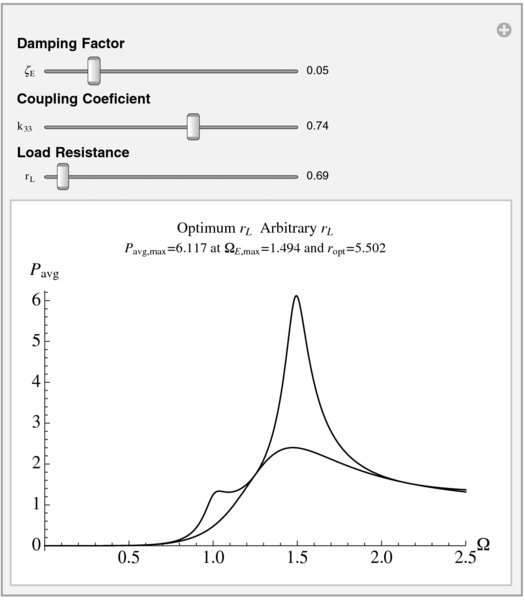
Figure 8.4 Initial configuration of the interactive graph to determine the normalized average power from a single degree-of-freedom piezoelectric energy harvester
Manipulate[
(* Determine maximum power with Eq. (8.15) substituted in Eq. (8.14) *)
   pmax=NMaximize[{pavg[x,ζ,k33,ropt[x,ζ,k33]],
      2.5>=x>=1.06},x];
(* Plot results *)
   Plot[{pavg[Ω,ζ,k33,ropt[Ω,ζ,k33]],pavg[Ω,ζ,k33,rL]},
      {Ω,0,2.5},PlotRange->{{0,2.5},All},
      PlotLabel->Column[{lab1,Row[{"Pavg,max=",
      NumberForm[pmax[[1]],4]," at ΩE,max=",
      NumberForm[Ω/.pmax[[2]],4]," and ropt=",
      NumberForm[ropt[Ω/.pmax[[2]],z,k33],4]}]},Center],
      AxesLabel->{Ω,"Pavg"},LabelStyle->{14},
      PlotStyle->{Black,Blue}],
(* Create sliders *)
   Style["Damping Factor",Bold],
   {{ζ,0.05,"ζE"},0.01,0.25,0.01,Appearance->"Labeled"
      ControlType->Slider},
   Style["Coupling Coeficient",Bold],
   {{k33,0.74,"k33"},0.5,0.9,0.01,Appearance->"Labeled",
      ControlType->Slider},
   Style["Load Resistance",Bold],
   {{rL,0.69,"rL"},0.01,20,0.01,Appearance->"Labeled",
      ControlType->Slider},
   Delimiter,
(* Create portions of a plot label *)
   Initialization:>(lab1=Row[{Style["Optimum rL",Black,14],
      Style[" Arbitrary rL",Blue,14]}];
(* Function representing Eq. (8.15) *)
      ropt[Ω_,ζ_,k33_]:=(ke2=k33^2/(1-k33^2);
         1/Ω Sqrt[(Ω^4+(4 ζ^2-2) Ω^2+1)/
         (Ω^4+(4 ζ^2-2 (1+ke2)) Ω^2+(1+ke2)^2)]);
(* Function representing Eq. (8.14) *)
      pavg[Ω_,ζ_,k33_,rL_]:=(ke2=k33^2/(1-k33^2);
         0.5 Ω^6 rL ke2/((1-Ω^2 (1+2 ζ rL))^2+
            (Ω (2 ζ+rL (1+ke2)-rL Ω^2))^2));),
   TrackedSymbols:>{ζ,k33,rL}]
8.3 Two Degrees-of-Freedom Systems
8.3.1 Governing Equations
Consider a single degree-of-freedom system composed of a mass m1, a viscous damper with damping coefficient c1, and a spring with stiffness k1. Another single degree-of-freedom system composed of a mass m2, a viscous damper with damping coefficient c2, and a spring with stiffness k2 is attached to m1. The nondimensional governing equations of motion of a two degrees-of-freedom systems are given in Example 4.30 and, for convenience, are repeated here. Thus,
where
and fl(τ), l = 1, 2 is the force applied to mass ml.
8.3.2 Response to Harmonic Excitation: Amplitude Response Functions
It is assumed that the applied force is harmonic and of the form fl(τ) = FlejΩτ, l = 1, 2. Then, if it is assumed that a solution to Eq. (8.16) is of the form xl(τ) = XlejΩτ, it is found that

where Ω = ω/ωn1, and
For Eq. (8.17), two scenarios are considered: (i) F1 ≠ 0 and F2 = 0 and (ii) F2 ≠ 0 and F1 = 0. For these assumptions, it is found that the frequency-response functions are
where, in Hij, the subscript i refers to the response of mass mi and the subscript j indicates that the force is applied to mj. The magnitudes of the frequency response functions are given by |Hij|.
The natural frequencies of the systems are determined by finding the values of Ω that satisfy D(Ω) = 0 when ζ1 = ζ2 = 0. These operations yield

The magnitudes of the frequency response functions |Hij| and the natural frequencies Ω1,2 are placed in an interactive environment shown in Figure 8.5, where the effects that the parameters ωr, mr, ζ1, and ζ1 can have on these quantities are displayed. The option of filling the region under each curve has also been provided.

Figure 8.5 Initial configuration of the interactive graph to determine the magnitudes of the amplitude response functions of a two degrees-of-freedom system. Also displayed are the system’s natural frequencies
The program that creates this interactive environment is as follows.
Manipulate[mr=mr ; Ωr=wr; a1=1+wr^2 (1+mr);
(* Eq. (8.20) *)
   Ω1=Sqrt[0.5 (a1-Sqrt[a1^2-4 Ωr^2])];
    Ω2=Sqrt[0.5 (a1+Sqrt[a1^2-4 Ωr^2])];
(* Red dashed lines for display *)
   ws={{{Red,Dashed,Line[{{Ω1,0},{Ω1,100}}]}},
      {{Red,Dashed,Line[{{Ω2,0},{Ω2,300}}]}}};
(* Results displayed in a 2-by-2 graphics grid *)
   plt[n_]:=Plot[Hij[Ω][[n]],{Ω,0.0,2.5},
      AxesLabel->{"Ω",lab[[n]]},PlotRange->{{0,2.5},All},
      PlotStyle->Blue,LabelStyle->{14},
      Filling->If[fill==2,Axis,False],Epilog->ws];
   GraphicsGrid[{{plt[1],Style[Column[
         {Row[{"Ω1=", NumberForm[Ω1,3]}],
         Row[{"Ω2=",NumberForm[Ω2,4]}]}],16,Red]},
            {plt[2],plt[3]}}],
(* Create sliders *)
   Style["System Parameters", Bold],
   {{ζ1,0.14,"ζ1"},0,0.4,0.01,Appearance->"Labeled",
      ControlType->Slider},
   {{ζ2,0.07,"ζ2"},0,0.4,0.01,Appearance->"Labeled",
      ControlType->Slider},
   {{mr,0.6,"mr"},0.01,1.2,0.01,Appearance->"Labeled",
      ControlType->Slider},
   {{wr,0.9,"Ωr"},0.01,1.5,0.01,Appearance->"Labeled",
      ControlType->Slider},
   Delimiter,
   Style["Curve Fill",Bold],
   {{fill,2," "},{1->"None",2->" Fill "},
      ControlType->SetterBar},
(* Place controls at left *)
   ControlPlacement-> Left,
   TrackedSymbols:>{ζ1,ζ2,mr,wr,fill},
   Initialization:>(lab={"H11","H12 = H21","H22"};
(* Function representing the absolute value of Eq. (8.19). *)
(* Output is a 3-element list *)
   Hij[Ω_]:=(
      den=Ω^4-I (2 ζ1+2 ζ2 mr Ωr+2 ζ2 Ωr) Ω^3-(1+mr Ωr^2+Ωr^2+
         4 ζ1 ζ2 Ωr) Ω^2+I (2 ζ2 Ωr+2 ζ1 Ωr^2) Ω+Ωr^2;
      h22=Abs[(-Ω^2+2 I (ζ1+ζ2 mr Ωr) Ω)/den/mr];
      h12=Abs[(2 I ζ2 mr Ωr Ω+mr Ωr^2)/den/mr];
      h11=Abs[(-Ω^2+2 I ζ2 Ωr Ω+Ωr^2)/den];
      {h11,h12,h22});
8.3.3 Enhanced Energy Harvester
We shall create an enhanced energy harvester by replacing the spring k2 in the two degrees-of-freedom system given by Eq. (8.16) with a piezoelectric element as defined in Section 8.2.4. The output of this element is connected to a load resistor RL. In addition, the base that is supporting k1 and c1 is now assumed to move an amount x3. Then, in Eq. (8.16), the base excitation can be accounted if f2 = 0 and f1 is replaced with
If harmonic excitation of the form xl(τ) = XlejΩτ, l = 1, 2, 3, is assumed, it can be shown that the normalized average power P′avg(Ω) into the load resistor can be written as [2, Section 2.7.3]
where ![]() ,
,
and

It can be shown that the maximum average power at a given frequency can be obtained when r′L = r′L, opt, which is determined from

Thus, at a given value of Ω, any value of r′L that is different from r′L, opt will result in less average power. However, this value of r′L, opt does not necessarily give the largest maximum average power. That has to be determined numerically.
We shall create an interactive environment shown in Figure 8.6 that plots P′avg(Ω) for the optimum value r′L, opt at each value of Ω and allows one to explore this curve as a function of ωr, mr, ζ1, ζ2, and k33. For each set of these parameters, the maximum average power, the frequency at which it occurs, and the corresponding value of r′L are determined and displayed. In addition, we have included for comparison purposes the equivalent curve for the single degree-of-freedom system, which are given by Eqs. (8.14) and (8.15). To compare the notation of the two degrees-of-freedom energy harvester with that of the single degree-of-freedom energy harvester, we note the following: ωn = ω2n, Yo = X3, ζE = ζ2, and ΩE = Ω/ωr. The program that creates this interactive environment is as follows.
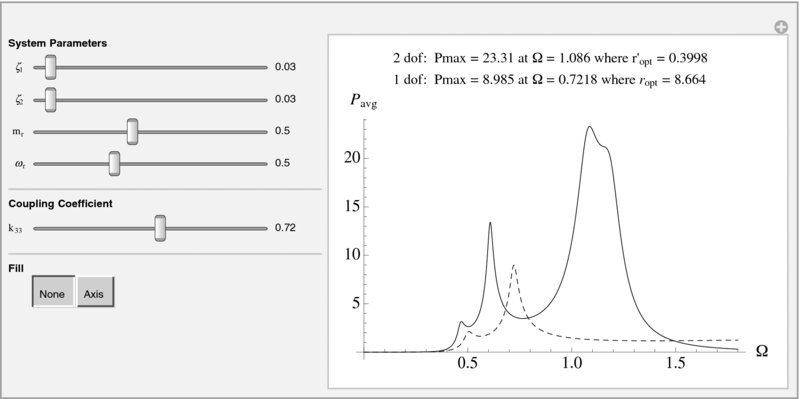
Figure 8.6 Initial configuration of the interactive graph to determine the maximum average power from an enhanced piezoelectric energy harvester and from a single degree-of-freedom energy harvester
Manipulate[Ωr=wr;   mr=mr;   ke2=k33^2/(1-k33^2);
   pt=pavg2[rvv,rLopt[rvv]];
   lb=First[Ordering[pt,-1]];
(* Maximum average power from two degrees-of-freedom system *)
   rx=Quiet[FindMaximum[pavg2[Om2,rLopt[Om2]],
      {Om2,rvv[[lb]]}]];
   Omax=Om2/.Last[rx]; ropt2=rLopt[Omax];
   pt1=pavg1[rvv/Ωr,rLopt1[rvv/Ωr]];
   lb1=First[Ordering[pt1,-1]];
(* Maximum average power from single degree-of-freedom system *)
   rx1=Quiet[FindMaximum[{pavg1[Om1/Ωr,rLopt1[Om1/Ωr]],
      {0<Om1<1.8}},{Om1,rvv[[lb1]]}]];
   Omax1=Om1/.Last[rx1];
   ropt11=rLopt1[Omax1/wr];
(* Plot results *)
   Plot[{pavg2[x,rLopt[x]],pavg1[x/Ωr,rLopt1[x/Ωr]]},
      {x,0,1.8},Filling->fill,PlotRange->All,
      AxesLabel->{Ω,"Pavg"},LabelStyle->14,
      PlotStyle->{Blue,{Red,Dashed}},
      PlotLabel->Column[{Style[Row[
         {lab2,NumberForm[First[rx],4]," at Ω = ",
         NumberForm[Omax, 4],lab4,NumberForm[ropt2,4]}],
         Blue,12],Style[Row[{lab3,NumberForm[First[rx1],4],
      " at Ω = ",NumberForm[Omax1,4],lab5,
         NumberForm[ropt11,4]}], Red,12]}]],
(* Create sliders and setter bar *)
   Style["System Parameters",Bold],
   {{ζ1,0.03,"ζ1"},0.02,0.35,0.01,Appearance->"Labeled",
      ControlType->Slider},
   {{ζ2,0.03,"ζ2"},0.02,0.35,0.01,Appearance->"Labeled",
      ControlType->Slider},
   {{mr,0.5,"mr"},0,1.2,0.01,Appearance->"Labeled",
      ControlType->Slider},
   {{wr,0.5,"Ωr"},0,1.5,0.01,Appearance->"Labeled",
      ControlType->Slider},
   Delimiter,
   Style["Coupling Coefficient",Bold],
   {{k33,0.72,"k33"},0.5,0.9,0.01,Appearance->"Labeled",
      ControlType->Slider},
   Delimiter,
   Style["Fill",Bold],
   {{fill,None," "},{None,Axis},ControlType->SetterBar},
   TrackedSymbols:>(ζ1,ζ2,mr,wr,fill,k33},
(* Create labels, a list of numbers, and several functions *)
   Initialization:>(lab2="2 dof: Pmax = ";
      lab3="1 dof: Pmax = ";    lab4=" where r′opt = ";
      lab5=" where ropt = ";    rvv=Range[0.01,1.8,0.01];
(* Function representing Eqs. (8.22) and (8.23). *)
(* Output is a 5-element list. *)
   fgc[Ω_]:=(a33=ke2 Ωr^2 mr; cC=Ωr^2+2 I ζ2 Ωr Ω;
      aA=-Ω^2+1+mr Ωr^2+2 I (ζ1+ζ2 mr Ωr) Ω;
      bB=mr Ωr^2+2 I ζ2 mr Ωr Ω; eE=-Ω^2+Ωr^2+2 I ζ2 Ωr Ω;
      co=0.5 ke2/Ωr Abs[I Ω (1+2 I ζ1 Ω) (Re[cC]-Re[eE]+
         I (Im[cC]-Im[eE]))]^2;
      f1=Ω ((Im[bB]-Im[aA]) a33/mr+Im[bB] Re[cC]+
         Re[bB] Im[cC]-Im[aA] Re[eE]-Re[aA] Im[eE]+
         (Im[cC]-Im[eE]) a33);
      f2=Im[bB] Im[cC]-Re[bB] Re[cC]-
         Im[aA] Im[eE]+Re[aA] Re[eE];
      g1=Ω ((Re[aA]-Re[bB]) a33/mr+Im[bB] Im[cC]-
         Re[bB] Re[cC]-Im[aA] Im[eE]+Re[aA] Re[eE]+
         (Re[eE]-Re[cC]) a33);
      g2=Im[aA] Re[eE]-Re[bB] Im[cC]-Im[bB] Re[cC]+
         Re[aA] Im[eE]; {f1,f2,g1,g2,co});
(* Function representing Eq. (8.21) *)
   pavg2[Ω_,rL_]:=(q=fgc[Ω];
      rL q[[5]]/Abs[q[[1]] rL+q[[2]]+I (q[[3]] rL+q[[4]])]^2);
(* Function representing Eq. (8.24) *)
   rLopt[Ω_]:=(q=fgc[Ω];
      Sqrt[(q[[2]]^2+q[[4]]^2)/(q[[1]]^2+q[[3]]^2)]);
(* Function representing Eq. (8.15) *)
   rLopt1[Ω_]:=(1/Ω Sqrt[(Ω^4+(4 ζ2^2-2) Ω^2+1)/
      (Ω^4+(4 ζ2^2-2 (1+ke2)) Ω^2+(1+ke2)^2)]);
(* Function representing Eq. (8.14) *)
   pavg1[Ω_,rL_]:=(aR=1-Ω^2 (1+2 ζ2 rL);
      bR=Ω (2 ζ2+rL (1+ke2)-rL Ω^2);
      0.5 Ω^6 rL ke2/(aR^2+bR^2));)]
8.4 Thin Beams
8.4.1 Natural Frequencies and Mode Shapes of a Cantilever Beam with In-Span Attachments
A cantilever beam of constant cross section has a length L (m), cross-sectional area A (m2), area moment of inertia I (m4), Young’s modulus E (N·m−2), and density ρ (kg·m−3). There are two in-span attachments: one is a mass Mi (kg) that is attached at x = Lm, 0 < Lm ≤ L and the other is a translation spring of stiffness ki (N·m−1) that is attached at x = Ls, 0 < Ls ≤ L. It is mentioned that, in general, Lm and Ls are independent; however, only the case for Lm = Ls will be considered here.
The natural frequency coefficients Ωn for the case where ηs = ηm are determined from [2, Section 3.3.3]
where

and
In addition,

It is noted that when Ki → ∞, we have the case of a beam with an intermediate rigid support for which the displacement is zero but the rotation is unrestrained.
The mode shapes are given by
where u(η) is the unit step function. The normalized mode shape is given by Yn(η)/max |Yn(η)|. The node points are those values of η for which
To improve the numerical evaluation process, the magnitude of Ki appearing in Eq, (8.25) is monitored. Whenever the value exceeds 500, the equation is first divided by Ki and then numerically evaluated.
An interactive environment shown in Figure 8.7 is created to explore the effects of attachments on the lowest four natural frequencies and their associated mode shapes and node points. The program that creates Figure 8.7 is as follows.
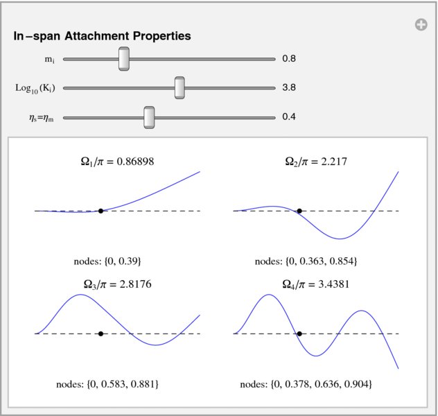
Figure 8.7 Initial configuration of the interactive graph to obtain the natural frequencies, modes shapes, and node points of a cantilever beam for various combinations of in-span attachments
Manipulate[Ki=10^kKi; w=ce8[Ωe]; nf={};
(* Determine ![]() n from Eq. (8.25) *)
n from Eq. (8.25) *)
   Do[If[w[[n]] w[[n+1]]<0,AppendTo[nf,
      (x/.Quiet[FindRoot[ce8[x],{x,Ωe[[n]], Ωe[[n+1]]}]])/π];
      If[Length[nf]==4,Break[]]],{n,1,Length[w]-1,1}];
(* Determine node points from Eq. (8.30) *)
      node={}; mss={};
      Do[npt={}; ms1=shapeIns8[etta,nf[[nct]] π];
      ms1=ms1/Max[Abs[ms1]];
         Do[If[ms1[[nv]] ms1[[nv+1]]<0,
         AppendTo[npt,y/.Quiet[FindRoot[
            shapeIns8[y,nf[[nct]] π],{y,etta[[nv]],
            etta[[nv+1]]}]]]],{nv,1,le-1,1}]; AppendTo[mss,ms1];
         PrependTo[npt,0]; AppendTo[node,npt],{nct,1,4}];
   ypot={etas (le-1)+1,0};
(* Plot results on a 2×2 grid *)
   GraphicsGrid[{{plt[mss[[1]],1,le,node[[1]],ypot,nf[[1]]],
      plt[mss[[2]],2,le,node[[2]],ypot,nf[[2]]]},
      {plt[mss[[3]],3,le,node[[3]],ypot,nf[[3]]],
      plt[mss[[4]],4,le,node[[4]],ypot,nf[[4]]]}}],
(* Create Sliders *)
   Style["In-span Attachment Properties",Bold,11],
   {{mi,0.8,"mi"},0.0,3,0.1,
      Appearance->"Labeled",ControlType->Slider},
   {{kKi,3.8,"Log10(Ki)"},-4,10,0.1,
      Appearance->"Labeled",ControlType->Slider},
   {{etas,0.4,"[ηs=[ηm"},0.01,0.99,0.01,
      Appearance->"Labeled",ControlType->Slider},
   TrackedSymbols:>{mi,kKi,etas},
   Initialization:>(Ωe=Range[0.001,25.,0.1];
      etta=Range[0,1,0.01]; le=Length[etta];
(* Functions representing Eq. (8.27) *)
      Q[Ω_,y_]:=(Cos[Ω y]+Cosh[Ω y])/2.;
      R[Ω_,y_]:=(Sin[Ω y]+Sinh[Ω y])/2.;
      S[Ω_,y_]:=(-Cos[Ω y]+Cosh[Ω y])/2.;
      T[Ω_,y_]:=(-Sin[Ω y]+Sinh[Ω y])/2.;
(* Functions representing Eq. (8.26) *)
      d3[Ω_,y_]:=R[Ω,y] T[Ω,y]-Q[Ω,y]^2;
      h3[Ω_,x_,y_]:=T[Ω,x] (T[Ω,1] R[Ω,1-y]-Q[Ω,1] Q[Ω,1-y])+
         S[Ω,x] (R[Ω,1] Q[Ω,1-y]-Q[Ω,1] R[Ω,1-y]);
(* Function representing Eq. (8.25) *)
      ce8[Ω_]:=If[Ki<500.,d3[Ω,1]-(Ki-mi Ω^4) h3[Ω,etas,etas]/
         Ω^3, d3[Ω,1]/Ki-(1.-mi Ω^4/Ki) h3[Ω,etas,etas]/Ω^3];
(* Function representing Eq. (8.29) *)
      shapeIns8[[η_,Ω_]:=-T[Ω,[η-etas] d3[Ω,1] UnitStep[[η-etas]+
         h3[Ω,[η,etas];
(* Plotting function *)
      plt[f_,n1_,le_,nod_,ypot_,freq_]:=
         ListLinePlot[f, Axes->False,PlotLabel->Row[{"Ω"n1,"/π=",
            NumberForm[freq,5]}],PlotRange->{{1,le},{-1.5,1.1}},
            Epilog->{{Black,Dashed,Line[{{1,0},{le,0}}]},
            {Inset[Style[Row[{"nodes: ",NumberForm[nod,3]}],10],
            {45,-1.3}]},{PointSize[Medium],Red,Point[ypot]}}];)]
8.4.2 Effects of Electrostatic Force on the Natural Frequency and Stability of a Beam
We shall examine a beam clamped at both ends and a cantilever beam when each beam is subjected to an electrostatic force. The electrostatic force field can include a fringe correction factor. In addition, for the beam clamped at both ends two additional effects will be taken into account. One is due to the application of an externally applied in-plane tensile force po. The second is to include in-plane stretching due to the transverse displacement.
Consider a beam of constant cross section of length L (m), cross-sectional area A (m2), moment of inertia I (m4), Young’s modulus E (N·m−2), and density ρ (kg·m−3). The cross section of the beam is rectangular with a depth of h and a width b. The bottom surface of the beam is parallel to a fixed, flat surface that is a distance do from it. A voltage of magnitude Vo is applied across the gap do, which forms an electrostatic field. If the transverse displacement of the beam is w and no transverse force other than the electrostatic force is applied, then an estimate for the lowest natural frequency assuming small oscillations at frequency ω about a static equilibrium position denoted ϕs is given by [2, Section 4.3.3]
where
and Ω = ωto where to is defined in Eq. (8.28). In Eq. (8.32), we have for a beam clamped at both ends

and for a cantilever beam
Furthermore, the following definitions have been introduced
In Eq. (8.35), ![]() o is the permittivity of free space, which for air is 8.854 × 10⁻¹² F·m−1, and c3 is the fringe correction factor. When the fringe correction is ignored, c3 = 0. The effects of the displacement-induced in-plane stretching become negligible as dr → 0.
o is the permittivity of free space, which for air is 8.854 × 10⁻¹² F·m−1, and c3 is the fringe correction factor. When the fringe correction is ignored, c3 = 0. The effects of the displacement-induced in-plane stretching become negligible as dr → 0.
In Eq. (8.31), there are two interdependent quantities that have to be determined: ϕs and ![]() . First, we need to determine the value of E1Vo, denoted (E1Vo)PI, at which the system becomes unstable. Corresponding to this value is the maximum static equilibrium value denoted ϕs,PI and the maximum displacement denoted
. First, we need to determine the value of E1Vo, denoted (E1Vo)PI, at which the system becomes unstable. Corresponding to this value is the maximum static equilibrium value denoted ϕs,PI and the maximum displacement denoted ![]() . For a beam clamped at both ends,
. For a beam clamped at both ends, ![]() and for a cantilever beam
and for a cantilever beam ![]() . The procedure to determine these values is as follows. We first determine ϕs, PI from the solution to
. The procedure to determine these values is as follows. We first determine ϕs, PI from the solution to
where
and Y is given by Eq. (8.33) or Eq. (8.34) as the case may be. Then, (E1Vo)PI is determined from

Next, we evaluate Eq. (8.32) by first assuming a value for E1Vo in the range 0 < E1Vo < (E1Vo)PI. Then, for this value of E1Vo the value of ϕs that satisfies
is determined. Substituting ϕs into Eq. (8.32) and the result in turn into Eq. (8.31), we obtain the value of Ω2.
An interactive environment shown in Figure 8.8 is created to explore the effects that the boundary conditions, the in-plane loading, the fringe correction factor and beam geometry, and displacement-induced in-plane stretching have on the first natural frequency coefficient. This program is computationally intensive and, therefore, has a very long delay from the time a parameter is changed until the graph is drawn. To overcome this, we have set ContinuousAction to False and used the general form of the slider so that it is also possible to enter the values directly. Additionally, FindRoot internally does some symbolic operations, which cause difficulty when interacting with NIntegrate via gr and dgr. Therefore, as discussed in Sections 5.2 and 5.5, the inputs to these functions are restricted to numerical values by checking the input with ?NumericQ and by selecting the method used by NIntegrate to forego any symbolic operations, which is done by setting SymbolicProcessing to False.

Figure 8.8 Initial configuration of the interactive graph to determine the lowest natural frequency of a beam subject to an electrostatic force, in-plane load, and displacement-induced in-plane force
The program that creates Figure 8.8 is as follows.
Manipulate[
(* Obtain parameters in Eqs. (8.33) to (8.35) *)
   If[fe==1,c3=(0.204+0.6 hb^0.24) (hb/hdo)^0.76,c3=0];
   If[bc==1,mo=1./630.;k=0.8+So 2./105.;
   If[inpl==1,k1=6./hdo^2 (2/105)^2,k1=0],
      mo=104./45.;k=144./5;k1=0];
   If[bc==1,If[So==0,yMax=26,yMax=40],yMax=4];
   If[bc==1,loc=1,loc=0.1];
(* Create figure for insertion into main figure *)
   If[fe==1,plin=ListLinePlot[{{{0,0},{h/hb,0}},{{0,h/hdo},
      {h/hb,h/hdo},{h/hb,h/hdo+h},{0,h/hdo+h},{0,h/hdo}}},
      Axes->False,PlotRange->{{0,5.1},{-0.1,4.4}},
      ImageSize->Tiny,PlotStyle->{{Black},{Black}}],
      plin=""];
(* Solve Eqs. (8.36) and (8.38) *)
   If[bc==1,guess=8.5;pe=11.5,guess=0.08;pe=0.3];
   phiPI=phi/.FindRoot[gr[phi] (k+3. k1 phi^2)
      -dgr[phi] (k phi+k1 phi^3),{phi,guess,0.01,pe}];
   eVPI=Sqrt[(k phiPI+k1 phiPI^3)/gr[phiPI]];
   If[bc==1,yPI=phiPI/16.,yPI=3. phiPI];
(* Plot results *)
   Plot[freq2[x],{x,0.0,0.995 eVPI},
      PlotRange->{{0,Ceiling[eVPI]},{0,yMax}},
      MaxRecursion->2,PlotPoints->25,AxesLabel->{"E1Vo","Ω2"},
      PlotLabel->Row[{lab1,NumberForm[eVPI,4],lab2,
      NumberForm[yPI,3]}],Epilog->{{Dashing[Medium],Red,
         Line[{{eVPI,0},{eVPI,yMax}}]},
      Inset[plin,{loc,loc},{0,0}]}],
(* Create sliders and radio buttons *)
   Style["Beam Boundary Conditions",Bold],
   {{bc,1," "},{1->"Clamped-Clamped",2->"Cantilever"},
      ControlType->RadioButtonBar},
   Delimiter,
   Style["In-Plane Stretching and Fringe Effects",Bold],
   {{fe,1,"Include Fringe Effects?"},
   {1->"Yes",2->"No"},ControlType->RadioButtonBar},
   {{inpl,1,"Include In-Plane Stretching?"},
      {1->"Yes",2->"No"},ControlType->RadioButtonBar,
      Enabled->If[bc==1,True,False]},
   Delimiter,
   Style["Beam Cross Section (Required for Fringe
      Effects)",Bold],
   {{hb,2,"h/b"},0.2,2,0.1,Appearance->{"Labeled","Open"},
      Enabled->If[fe==1,True,False],ControlType->Slider,
      ContinuousAction->False},
   {{hdo,0.5,"h/do"},0.5,5,0.1,ContinuousAction->False,
      Appearance->{"Labeled","Open"},ControlType->Slider,
      Enabled->If[fe==1,True,False]},
   Delimiter,
   Style["Applied Axial Tensile Force",Bold],
   {{So,0,"So"},0,80,5,ContinuousAction->False,
      Appearance->{"Labeled","Open"},ControlType->Slider,
      Enabled->If[bc==1,True,False]},
   ControlPlacement->Left,
   Initialization:>{lab1="(E1Vo)PI ≈ "; lab2=" yPI ≈ "; h=1;
(* Functions representing Eqs. (8.37) and (8.32) *)
   gr[phi_?NumericQ]:=Module[{aa},
      If[bc==1,yY=aa^2 (aa-1)^2,yY=(aa^2 (aa^2-4 aa+6))];
      Quiet[NIntegrate[yY/(1-yY phi)^2+c3 yY/
         (1-yY phi)^1.24,{aa,0,1},MaxRecursion->3,
         Method->{Automatic,
         "SymbolicProcessing"->False}]]];
   dgr[phi_?NumericQ]:=Module[{aa},
      If[bc==1,yY=aa^2 (aa-1)^2,yY=(aa^2 (aa^2-4 aa+6))];
      Quiet[NIntegrate[2.yY^2/(1-yY phi)^3+1.24 c3 yY^2/
         (1-yY phi)^2.24,{aa,0,1},MaxRecursion->3,
         Method->{Automatic,
            "SymbolicProcessing"->False}]]];
(* Function that solves Eq. (8.39) *)
      phiStatic[eV_?NumericQ]:=(If[bc==1,gues=5.,gues=0.1];
         phix/.Quiet[FindRoot[k phix+k1 phix^3-eV^2 gr[phix],
            {phix,gues}]]);
(* Function representing Eq. (8.31) *)
      freq2[eV_]:=(phiStat=phiStatic[eV];
         Sqrt[(k+3 k1 phiStat^2-eV^2 dgr[phiStat])/mo]);},
   TrackedSymbols:>{bc,inpl,fe,hb,hdo,So}]
8.4.3 Response of a Cantilever Beam with an In-Span Attachment to an Impulse Force
We shall use the results of Section 8.4.1 and the program presented therein to examine the response a cantilever beam of length L to an impulse force at x = L1. At x = Ls, 0 ≤ Ls ≤ L, a spring with spring constant ki is attached. The response of this system is given by [2, Section 3.10.3]
where Yn(η) is given by Eq. (8.29), τ = t/to, where to is given by Eq. (8.28), η1 = L1/L, 0 ≤ η1 ≤ 1, is the location of the impulse, Ωn are solutions to Eq. (8.25), and
An interactive environment shown in Figure 8.9 is created to explore the effects that various attachments and point of application of an impulse force have on the spatial and temporal response of a cantilever beam. Eight mode shapes are used in Eq. (8.40).

Figure 8.9 Initial configuration of the interactive graph to determine the response of a cantilever beam with an in-span attachment to an impulse force at η1
The program that creates Figure 8.9 is as follows.
Manipulate[Ki=10^kKi;
(* Obtain lowest eight natural frequencies *)
   w=ce8[Ωe]; nf={};
   Do[If[w[[n]] w[[n+1]]<0,
      AppendTo[nf,(x/.Quiet[FindRoot[ce8[x],
         {x,Ωe[[n]],Ωe[[n+1]]}]])];
      If[Length[nf]==nroot,Break[]]],{n,1,Length[w]-1,1}];
(* Evaluate Eq. (8.41) *)
   nsubn=Table[NIntegrate[shapeIns8[x,nf[[n]]]^2,{x,0,1}]+
         mR shapeIns8[1,nf[[n]]]^2,{n,1,nroot}];
(* Evaluate Eq. (8.40) *)
   ta=Range[0,tend,tend/40.];
   yet=Table[Table[{τ,[η,Total[-shapeIns8[[η,nf]*
      shapeIns8[eta1,nf] Sin[nf^2 τ]/(nf^2 nsubn)]},
      {τ,ta}],{[η,et}];
   ListPlot3D[Flatten[yet,1],Mesh->{40,20},
      ViewPoint->{-1.3,-2,2},AxesLabel->{"τ","[η"," y([η,τ)"}],
(* Create sliders and radio buttons *)
   Style["Boundary Attachments at Right End",Bold],
   {{kKR,1.5,"Log10(KR)"},-5,12,0.1,Appearance->"Labeled",
      ControlType->Slider,ContinuousAction->False},
   {{mR,0.3,"mR"},0,1,0.1,Appearance->"Labeled",
      ControlType->Slider,ContinuousAction->False},
   Delimiter,
   Style["In-Span Attachments",Bold],
   {{inspan,2," "},{1->"No",2->"Yes"},
      ControlType->RadioButtonBar},
   Delimiter,
   Style["In-span Attachment Properties",Bold],
   {{kKi,4.6,"Log10(Ki)"},-4,10,0.1,Appearance->"Labeled",
      ControlType->Slider,ContinuousAction->False},
   {{etas,0.73,"[ηs"},0.01,0.99,0.01,Appearance->"Labeled",
      ControlType->Slider,ContinuousAction->False},
   Delimiter,
   Style["Location of Impulse",Bold],
   {{eta1,0.6,"[η1]"},0.1,1.0,0.01,ControlType->Slider,
      Appearance->"Labeled",ContinuousAction->False},
   Delimiter,
   Style["Maximum Time Span",Bold],
   {{tend,0.5,"τend"},0.5,3,0.5,ControlType->Slider,
      Appearance->"Labeled",ContinuousAction->False},
(* Generate some numerical values *)
   TrackedSymbols:>{ kKi,etas,tend,eta1 },
   ControlPlacement->Left,
   Initialization:>(Ωe=Range[0.01,45.,0.1];
      etta=Range[0,1,0.01]; le=Length[etta]; nroot=8;
      et=Range[0,1,0.05];
(* Functions representing Eq. (8.27) *)
      Q[Ω_,y_]:=(Cos[Ω y]+Cosh[Ω y])/2.;
      R[Ω_,y_]:=(Sin[Ω y]+Sinh[Ω y])/2.;
      S[Ω_,y_]:=(-Cos[Ω y]+Cosh[Ω y])/2.;
      T[Ω_,y_]:=(-Sin[Ω y]+Sinh[Ω y])/2.;
(* Functions representing Eq. (8.26) *)
      d3[Ω_,y_]:=R[Ω,y] T[Ω,y]-Q[Ω,y]^2;
      h3[Ω_,x_,y_]:=T[Ω,x] (T[Ω,1] R[Ω,1-y]-Q[Ω,1] Q[Ω,1-y])+
         S[Ω,x] (R[Ω,1] Q[Ω,1-y]-Q[Ω,1] R[Ω,1-y]);
(* Functions representing Eq. (8.25) with mi = 0 *)
      ce8[Ω_]:=If[Ki<500.,d3[Ω,1]-Ki h3[Ω,etas,etas]/Ω^3,
         d3[Ω,1]/Ki-h3[Ω,etas,etas]/Ω^3]]);
(* Function representing Eq. (8.29) *)
      shapeIns8[[η_,Ω_]:=-T[Ω,[η-etas] d3[Ω,1] UnitStep[[η-etas]+
         h3[Ω,[η,etas]])]
References
- B. Balachandran and E. B. Magrab, Vibrations, 2nd edn, Cengage Learning, Ontario Canada, 2009.
- E. B. Magrab, Vibrations of Elastic Systems, Solid Mechanics and Its Applications 184, Springer Science+ Business Media B.V., New York, 2012.