
9
Statistics
9.1 Descriptive Statistics
9.1.1 Introduction
Descriptive statistics are used to describe the properties of data; that is, how their values are distributed. One class of descriptors is concerned with the location of where the data tends to aggregate as typically described by the mean, median, or root mean square (rms). A second class of descriptors is concerned with the amount of dispersion of the data as typically described by the variance (or standard deviation) or by its quartiles. A third class of descriptors is the shape of the data as typically indicated by its histogram and its closeness to a known probability distribution. The commands used to determine these statistical descriptors are introduced in this section.
9.1.2 Location Statistics: Mean[], StandardDeviation[], and Quartile[]
The location statistics that we shall illustrate are the mean, median, and rms values, respectively, which are determined from
Mean[dat]
Median[dat]
RootMeanSquare[dat]
where dat is a list of numerical values representing measurements from a random process.
To illustrate these and other statistical functions, we shall consider the following data
datex1={111.,103.,251.,169.,213.,140.,224.,205.,166.,202.,
  227.,160.,234.,137.,186.,184.,163.,157.,181.,207.,189.,
  159.,180.,160.,196.,82.,107.,148.,155.,206.,192.,180.,
  205.,121.,199.,173.,177.,169.,93.,182.,127.,126.,187.,
  166.,200.,190.,171.,151.,166.,156.,187.,174.,164.,214.,
  139.,141.,178.,177.,243.,176.,186.,173.,182.,164.,162.,
  235.,164.,154.,156.,124.,149.,147.,116.,139.,129.,152.,
  175.,164.,141.,155.};
which will be used here and, subsequently, in several tables and examples. When used in the following examples, we shall employ the shorthand notation
datex1={…};
Thus, to obtain, respectively, the mean, median, and rms values of datex1, we have
datex1={…}; (* Data given above *)
Print["mean = ",Mean[datex1]]
Print["median = ",Median[datex1]]
Print["rms = ",RootMeanSquare[datex1]]
which yield
mean = 168.663
median = 167.5
rms = 171.969
The dispersion measures that we shall illustrate are, respectively, the standard deviation and the quantiles, which are determined from
StandardDeviation[dat]
Quantile[dat,q]
Quartiles[dat]
where q is the qth quantile in dat. Quartiles gives the 1/4, 1/2, and 3/4 quantiles of dat. However, Quantile always gives a result that is equal to an element of the dat. In this regard, it is different from Quartiles. Thus, to obtain the standard deviation and the quartiles using the two different functions, we have
datex1={…}; (* Data given above *)
Print["std dev = ",StandardDeviation[datex1]]
Print["qtl = ",Quantile[datex1,{1/4,3/4}]]
Print["quart = ",Quartiles[datex1]]
which yield
std dev = 33.7732
qtl = {149.,187.}
quart = {150.,167.5,187.}
Before introducing the shape descriptors, we shall first introduce several continuous distribution functions.
9.1.3 Continuous Distribution Functions: PDF[] and CDF[]
If X is a random variable that belongs to probability distribution dist, then the probability density function (pdf), cumulative distribution function (cdf), mean value of the distribution (μ), and the variance of the distribution (σ2), respectively, are obtained from
pdf=PDF[dist,x]
cdf=CDF[dist,x]
mu=Mean[dist]
var=Variance[dist]
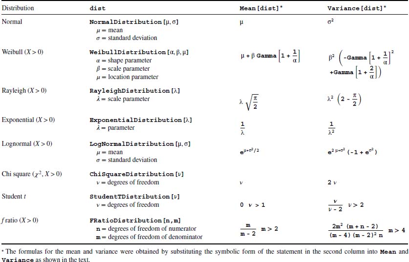
Several distributions commonly used in engineering and their corresponding Mathematica functions are given in Table 9.1. In addition, the formulas for the mean and variance for each distribution are also tabulated. If the arguments of dist are symbolic, then the results from these four functions are symbolic expressions. For example, if we use the Weibull distribution, then the following commands, respectively,
Table 9.1 Determination of the symbolic means and variances of selected probability distributions for the random variable X
Print["pdf = ",PDF[WeibullDistribution[α,β],x]]
Print["cdf = ",CDF[WeibullDistribution[α,β],x]]
Print["μ = ",Mean[WeibullDistribution[α,β]]]
Print["σ2 = ",Variance[WeibullDistribution[α,β]]]
yield, for x > 0,
ββααβαβ μβασβαα

If α and β are numerical values, then for, say, α = 2, β = 3, the probability that X = 1.5 is determined from
w=PDF[WeibullDistribution[2,3],1.5]
which gives w = 0.2596. To obtain a graph of the probability density function of the Weibull distribution for α = 2 and β = 3 and 0 ≤ X ≤ 6, we use
Plot[PDF[WeibullDistribution[2.,3.],x],{x,0,6},
  AxesLabel->{"x","Probability"}]
and obtain Figure 9.1.
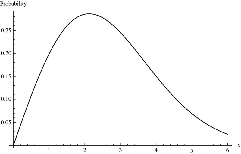
Figure 9.1 Wiebull probability density function for α = 2 and β = 3
9.1.4 Histograms and Probability Plots: Histogram[] and ProbabilityScalePlot[]
The shape visualization functions that we shall consider are
Histogram[dat,binspec,hspec]
ProbabilityScalePlot[dat,dist]
where dat is a list of numerical values representing measurements from a process and dist is the name of a distribution in quotation marks. The other quantities in Histogram are defined in Table 9.2. Histogram plots a histogram with its bins determined automatically and with any of several types of amplitudes for the y-axis. ProbabilityScalePlot plots dat on a probability scale that is specified by the probability distribution dist. If almost all the data values of dat lie on or are very close to the reference line that indicates that distribution’s variation with respect to X, then the data can be represented by that distribution. Some of the choices for the arguments of Histogram and ProbabilityScalePlot are summarized in Table 9.2.
Table 9.2 Histograms and probability graphs
| Plot type | Mathematica function |
| Histogram* | Histogram[dat,binspec,hspec,LabelingFunction->pos] dat = list of values binspec = Automatic – automatically selects number of bins (default) = n – specify number of bins hspec = "Count" – plots number of values in each bin (default) = "CumulativeCount" – plots the number of values in bin and preceding bins = "Probability" – plots fraction of number of values in each bin with respect to total number of values = "PDF" – plots probability density function : same as "Probability" = "CDF" – plots cumulative distribution function pos = position of where the labels are to appear: Top, Bottom, Left, Right, and Above |
| Probability | ProbabilityScalePlot[dat,dist] dat = list of values dist = "Normal" (default, if omitted) – plots dat assuming a normal distribution dist = "Weibull" – plots dat assuming a Weibull distribution dist = "Exponential" – plots dat assuming an exponential distribution dist = "LogNormal" – plots dat assuming a lognormal distribution dist = "Rayleigh" – plots dat assuming a Rayleigh distribution |
* The differences in using "Count" and "PDF" and using "CumulativeCount" and "CDF" are the units of the y-axis; for an equal number of bins, the shape of the histograms in each of these pairs is the same. See Table 9.3.
Examples of the effects that these arguments have on the vertical axes of the figures produced by Histogram are shown in Table 9.3. It is mentioned that when one passes the cursor over the bars in the histogram plot a tooltip appears that provides the height of that bar: either the number of samples or the fraction of the total number of samples depending on the plot options selected.
Table 9.3 Effects of several options of Histogram*

9.1.5 Whisker Plot: BoxWhiskerChart[]
Another way to visualize data in the aggregate is with a whisker plot. This type of display is useful when comparing two or more data sets. The command for this function is
BoxWhiskerChart[{dat1,dat2,…},specw,graph]
where datN are the lists of the data sets, specw is a specification for the specific form of the whisker plot, and graph are graphics-enhancement instructions. See the Documentation Center under the search entry BoxWhiskerChart for the details. We shall illustrate the use of BoxWhiskerChart for two data sets obtained by splitting datex1 in half. In addition, we shall use a notched whisker plot with its outliers appearing as blue dots, label each of the data sets, and give different colors to the boxes. Then,
datex1={…}; (* See Section 9.1.2 *)
BoxWhiskerChart[{datex1[[1;;40]],datex1[[41;;80]]},
  {"Notched",{"Outliers",Blue}},ChartStyle->{Red,Magenta},
  ChartLabels->{"Set 1","Set 2"}]
produces Figure 9.2. It is mentioned that when one passes the cursor over the figure a tooltip appears that provides the details of each whisker plot: maximum value, 75th quartile value, median, 25th quartile value, and minimum value. The maximum and minimum values include any outliers.
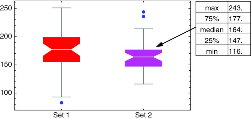
Figure 9.2 Enhanced notched whisker plot with outliers displayed. When the cursor is placed over each whisker plot, a Tooltip is displayed as shown in the figure for Set 2
9.1.6 Creating Data with Specified Distributions: RandomVariate[]
One can create a list of n data values (samples) that has a distribution given by dist, where dist is given by the distributions appearing in the second column1 of Table 9.1. The command that performs this operation is
data=RandomVariate[dist,n]
It is noted that each time this function is executed, the values of data will be different.
We shall create 300 samples from the Rayleigh distribution for λ = 80 and plot a histogram of these samples. On the histogram, the Rayleigh probability density function for this value of λ will be superimposed. In addition, an independent probability plot of the generated data set will be created. Then,
data=RandomVariate[RayleighDistribution[80.],300];
Show[Histogram[data,Automatic,"PDF",
  AxesLabel-> {"x","Probability"}],
  Plot[PDF[RayleighDistribution[80.],x],{x,0,300},
  PlotStyle->Black]]
ProbabilityScalePlot[data,"Rayleigh",
  FrameLabel->{"x","Rayleigh Probability"}]
When executed, this program yields Figure 9.3.

Figure 9.3 (a) Histogram of 300 data samples generated from the Rayleigh distribution compared to the Rayleigh probability density function (solid line); (b) Rayleigh probability plot of the 300 data samples
9.2 Probability of Continuous Random Variables
9.2.1 Probability for Different Distributions: NProbability[]
The probability P(X) that a continuous random variable X lies in the range x1 ≤ X ≤ x2, where x1 and x2 are from the set of all possible values of X, is defined as

where f(x) ≥ 0 for all x, and
The quantity f(x) is called the probability density function (pdf) for a continuous random variable.
The cumulative distribution function (cdf) F(x) is
and, therefore,
The determination of the numerical value of the probability that a random variable X lies within a specified range when X is a member of the probability distribution dist, is obtained from
NProbability[rng,x≈dist]
where rng is the range for which the probability is determined, dist is the distribution, and ≈ = ![]() dist
dist ![]() ; that is, ≈ is a representation for the sequential typing of the esc key followed by the four letters dist that is followed again by the typing of the esc key. The mathematical symbol ≈ will not work. Several of the distributions that can be used in this command are listed in the second column of Table 9.1.
; that is, ≈ is a representation for the sequential typing of the esc key followed by the four letters dist that is followed again by the typing of the esc key. The mathematical symbol ≈ will not work. Several of the distributions that can be used in this command are listed in the second column of Table 9.1.
NProbability can be used as a table of probabilities for various distributions. For example, if X is a random variable from the Weibull distribution for α = 1.5 and β = 3.7, then the probability that X ≥ 2 is obtained from
p=NProbability[x>=2.,x≈WeibullDistribution[1.5,3.7]]
which yields 0.672056. Thus, there is a 67% likelihood that the next sample will have a value greater than or equal to 2.
The probability from a set of data can be determined when the distribution is known (or can be assumed). For example, if it is assumed that datex1 of Section 9.1.2 can be approximated by a normal distribution, then we can use NProbability to estimate the probability that the next sample to be added to datex1 lies, say, between μ − 1.5σ ≤ X ≤ μ + 1.5σ, where μ is the mean and σ is the standard deviation. This probability estimate is obtained with
datex1={…}; (* See Section 9.1.2 *)
μ=Mean[datex1];
σ=StandardDeviation[datex1];
p=Probability[σ-1.5 σ<x<μ+1.5 σ, x≈NormalDistribution[μ,σ]]
The execution of this program gives 0.866386; that is, there is an 87% chance that the next sample will lie in the region indicated.
9.2.2 Inverse Cumulative Distribution Function: InverseCDF[]
Let us rewrite NProbability as
p=NProbability[ro(x,a),x≈dist]
where dist is the distribution and ro(x,a) is a relational operator that defines a region of x, the random variable, and the limit of that region is determined by a. One is often interested in the inverse of this function; that is, for a given distribution dist what is the value of a for a given value of p. The function that answers this question is
a=InverseCDF[dist,p]
The value of a is sometimes called the critical value for these stated conditions. The inverse function essentially replaces tables that typically appear in many statistics books.
To illustrate the use of InverseCDF, we shall consider the Student t distribution and determine the value of a for ν = 15 and a probability of p = 0.95. Then
a=InverseCDF[StudentTDistribution[15],0.95]
which gives a = 1.75305. To confirm that this is correct, we use
p=NProbability[x<=1.75305,x≈StudentTDistribution[15]]
and find that p = 0.95.
9.2.3 Distribution Parameter Estimation: EstimatedDistribution[] and FindDistributionParameters[]
For a given set of data and an assumption about the distribution of the data, it is possible to determine the parameters that govern that distribution. The parameters are determined in either of two ways. The first way, which is suitable for plotting, is
fcn=EstimatedDistribution[dat,dist[p1,p2,…]]
whose output is the function
dist[n1,n2,…]
In these expressions, dat is a list of data, pN are the parameters of the assumed distribution dist, and nN are the numerical values found by EstimatedDistribution for distribution dist. The values of nN are not accessible.
The second way to find the parameters is to use
para=FindDistributionParameters[dat,dist[p1,p2,…]]
where the output is of the form
{p1->n1,p2->n2,…}
In this case, the individual parameters are accessed by using p1/.para, etc.
To illustrate the use of these functions, we shall create 400 samples of data assuming a Weibull distribution and compare the parameters used to obtain these data with those obtained from FindDistributionParameters. Then
data=RandomVariate[WeibullDistribution[2.1,4.9,60],400];
fcn=EstimatedDistribution[data,WeibullDistribution[α, β, μ]]
para=FindDistributionParameters[data,
  WeibullDistribution[α, β, μ]]]
yield, respectively,
WeibullDistribution[1.74857,4.26186,60.4793]
and
{α->1.74857,β->4.26186,μ->60.4793}
In the first output, the values of α, β, and μ are inferred from their location in WeibullDistribution. In the second output, the values of α, β, and μ are accessible as follows: α = α/.para = 1.74857, β = β/.para = 4.26186, and μ =μ/.para = 60.4793.
9.2.4 Confidence Intervals: ⋅⋅⋅CI[]
Let θ be a numerical value of a statistic (e.g., the mean, variance, difference in means) of a collection of n samples. We are interested in determining the values of l and u such that the following is true
where 0 < α < 1. This means that we will have a probability of 1−α of selecting a collection of n samples that will produce an interval that contains the true value of θ. The interval
is called the 100(1−α)% two-sided confidence interval for θ.
The confidence limits depend on the distribution of the samples and on whether or not the standard deviation of the population is known. Several commonly used relationships to determine these confidence limits are summarized in Table 9.4. The quantities ![]() and s2, respectively, are the mean and variance for the sample values that are determined from Mean and Variance.
and s2, respectively, are the mean and variance for the sample values that are determined from Mean and Variance.
Table 9.4 Determination of the confidence intervals of several statistical measures

To illustrate several of these commands, we shall first determine the confidence interval at the 90% level of the mean of datex1 given in Section 9.1.2 when the variance is unknown. Then, from Case 1 of Table 9.4,
Needs["HypothesisTesting'"]
datex1={…}; (* See Section 9.1.2 *)
StudentTCI[Mean[datex1],
  StandardDeviation[datex1]/Sqrt[Length[datex1]],
  Length[datex1],ConfidenceLevel->0.90]
yields
{162.379,174.946}
Thus, the lower confidence limit at the 90% level is 162.379 and the upper confidence limit is 174.946.
For a second example, we shall determine the confidence at the 98% level for the difference in the means of two sets of data, set1 and set2, when the variances are unknown and unequal. Then, from Case 3 of Table 9.4,
set1={41.60,41.48,42.34,41.95,41.86,42.18,41.72,42.26,
  41.81,42.04};
set2={39.72,42.59,41.88,42.00,40.22,41.07,41.90,44.29};
MeanDifferenceCI[set1,set2,EqualVariances->False,
  ConfidenceLevel->0.98]
yields
{-1.29133,1.72183}
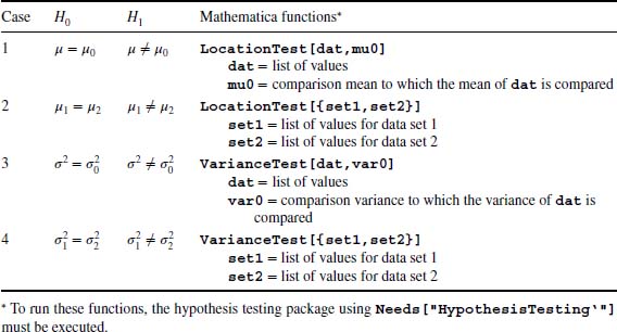
9.2.5 Hypothesis Testing: LocationTest[] and VarianceTest[]
Let θ be a numerical value of a statistic (e.g., the mean, variance, difference in means) of a collection of n samples. Suppose that we are interested in determining whether this parameter is equal to θo. In the hypothesis-testing procedure, we postulate a hypothesis, called the null hypothesis and denoted H0, and then based on the parameter θ form an appropriate test statistic q0. For testing mean values, q0 would be a t statistic, for variances it would be χ2, and for the ratio of variances it would be the f ratio statistic. We then compare the test statistic to a value that corresponds to the magnitude of the test statistic that one can expect to occur naturally, q. Based on the respective magnitudes of q0 and q, the null hypothesis is either accepted or rejected. If the null hypothesis is rejected, the alternative hypothesis denoted H1 is accepted. This acceptance or rejection of H0 is based on a quantity called the p-value, which is the smallest level of significance that would lead to the rejection of the null hypothesis. The percentage confidence level is 100(1 − p-value)%. Therefore, the smaller the p-value, the less plausible is the null hypothesis and the greater confidence we have in H1.
In Table 9.5, we have summarized several hypothesis-testing commands that are useful in engineering. The output of these commands is the p-value.
Table 9.5 Hypothesis testing of means and variances
We shall illustrate these commands with the following examples. Let us determine if there is a statistically significant difference at the 95% confidence level between the mean of datex1 given in Section 9.1.2 and a mean value of 174; that is, μ0 = 174. This is determined from Case 1 of Table 9.5. Thus,
datex1={…}; (* See Section 9.1.2 *)
p=LocationTest[datex1,174]
which yields that p = 0.161423. Since we can only be 100(1 − 0.161) = 83.6% confident, we do not reject H0. Recall from Section 9.1.2 that the mean value of these data is 168.7. However, if μ0 = 181, then we would find that p = 0.00161 and we are now 100(1 − 0.00161) = 99.84% confident that the mean of datex1 is different from a mean of 181.
For a second example, we determine whether the variances of data sets set1 and set2 of Section 9.2.4 are different. In this case, we use Case 4 of Table 9.5. Then,
set1={…}; set2={…} (* See Section 9.2.4 *)
p=VarianceTest[{set1,set2}]
gives that p = 0.0000653785 and we reject H0 with 99.993% confidence level that the variances are equal.
9.3 Regression Analysis: LinearModelFit[]
9.3.1 Simple Linear Regression2
Regression analysis is a statistical technique for modeling and investigating the relationship between two or more variables. A simple linear regression model has only one independent variable. If the input to a process is x and its response y, then a linear model is
where any regression model that is linear in the parameters βj is a linear regression model, regardless of the shape of the curve y that it generates. If there are n values of the independent variable xi and n corresponding measured responses yi, i = 1, 2, …, n, then estimates of y are obtained from
where xmin is the minimum value of xi, xmax is the maximum value of xi, and ![]() are estimates of βk.
are estimates of βk.
The function to determine ![]() is
is
modl=LinearModelFit[coord,{x,x^2,…},x,
  ConfidenceLevel->cl]
where coord = {{x1,y1},{x2,y2},…}, x is the independent variable, {x,x^2,…} matches the form of the independent variables in Eq. (9.1), and cl is the confidence level, which, if omitted is equal to 0.95. The output of LinearModelFit is the symbolic object of the form
FittedModel[b0+b1 x+b2 x^2+…]
where bK will be numerical values for the estimates ![]() . The access to numerous quantities that resulted from the statistical procedure used by LinearModelFit is obtained from
. The access to numerous quantities that resulted from the statistical procedure used by LinearModelFit is obtained from
modl["Option"]
where the choices for Option can be found in the Documentation Center under the search entry LinearModelFit.
Several of the more commonly used choices for Option are summarized in Table 9.6 for the case where
and the data set
Table 9.6 Several output quantities fromLinearModelFit for simple linear regression

xx={2.38,2.44,2.70,2.98,3.32,3.12,2.14,2.86,3.50,3.20,2.78,
    2.70,2.36,2.42,2.62,2.80,2.92,3.04,3.26,2.30};
yy={51.11,50.63,51.82,52.97,54.47,53.33,49.90,51.99,55.81,
    52.93,52.87,52.36,51.38,50.87,51.02,51.29,52.73,
    52.81,53.59,49.77};
pts=Table[{xx[[n]],yy[[n]]},{n,1,Length[xx]}];
We shall create a figure that plots pts, the fitted line, and the 90% confidence bands. Assuming that the above three definitions have been executed, the rest of the program is
modl=LinearModelFit[pts,{x},x,ConfidenceLevel->0.90];
bands=modl["MeanPredictionBands"];
xm=Min[xx]; xmx=Max[xx];
Show[Plot[modl[x],{x,xm,xmx},PlotStyle->Thick,
    AxesLabel->{"x","y(x)"}],
  ListPlot[pts,PlotMarkers->Automatic],
  Plot[{bands[[1]],bands[[2]]}/.x->f,{f,xm,xmx},
  PlotStyle->Dashing[Medium]]]
The results are shown in Figure 9.5.
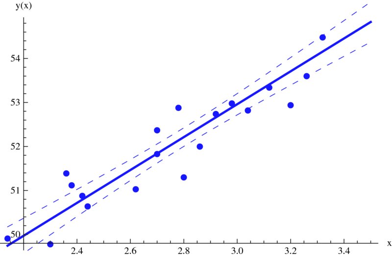
Figure 9.5 Straight line fit to data values shown and the 90% confidence bands of the fitted line
To determine if the residuals between the fitted curve and the original data are normally distributed, we plot them on a probability plot. If the residuals are close to the line representing a normal distribution, we can say that the fit is good. Thus,
ProbabilityScalePlot[modl["FitResiduals"],"Normal",
  PlotMarkers->Automatic,
  FrameLabel->{"Residual","Normal Probability"}]
produces Figure 9.6, which indicates that the fit is good.

Figure 9.6 Normal probability distribution plot of the residuals for the fit shown in Figure 9.5
9.3.2 Multiple Linear Regression
Multiple linear regression is similar to that for simple linear regression except that the form for the input to LinearModelFit is slightly different. Consider the output of a process y = y(x1, x2,…, xn), where xk are the independent input variables to that process. Then, for a specific set of values xk,m, m = 1, 2, … the output is ym. A general linear regression model for this system is of the form
where ![]() , p, s = 0, 1, 2, …, are independently chosen integers, but do not include the case p = s = 0.
, p, s = 0, 1, 2, …, are independently chosen integers, but do not include the case p = s = 0.
Then, for multiple regression analysis, an estimate of y and βk, denoted, respectively, ![]() and
and ![]() , are obtained from
, are obtained from
modlm=LinearModelFit[coord,{f1,f2,…},{x1,x2,…},
	   ConfidenceLevel->cl]
where coord={{x11,x21,…,y1},{x12,x22,…,y2},…}.
To illustrate multiple regression analysis, consider the data shown in Table 9.7. We shall fit these data with the following model
Table 9.7 Data for the multiple linear regression example

These data are converted to the form shown for coord above as follows
y={0.22200,0.39500,0.42200,0.43700,0.42800,0.46700,0.44400,
  0.37800,0.49400,0.45600,0.45200,0.11200,0.43200,0.10100,
  0.23200,0.30600,0.09230,0.11600,0.07640,0.43900,0.09440,
  0.11700,0.07260,0.04120,0.25100,0.00002};
x11={7.3,8.7,8.8,8.1,9.0,8.7,9.3,7.6,10.0,8.4,9.3,7.7,9.8,
  7.3,8.5,9.5,7.4,7.8,7.7,10.3,7.8,7.1,7.7,7.4,7.3,7.6};
x21={0.0,0.0,0.7,4.0,0.5,1.5,2.1,5.1,0.0,3.7,3.6,2.8,4.2,
  2.5,2.0,2.5,2.8,2.8,3.0,1.7,3.3,3.9,4.3,6.0,2.0,7.8};
x31={0.0,0.3,1.0,0.2,1.0,2.8,1.0,3.4,0.3,4.1,2.0,7.1,2.0,
  6.8,6.6,5.0,7.8,7.7,8.0,4.2,8.5,6.6,9.5,10.9,5.2,20.7};
coord=Table[{x11[[n]],x21[[n]],x31[[n]],y[[n]]},
  {n,1,Length[y]}];
Executing these statements, the multiple regression model is determined from
modlm=LinearModelFit[coord,{x1,x2,x3,x1 x2,x1 x3,x2 x3,
  x1^2,x2^2,x3^2},{x1,x2,x3},ConfidenceLevel->0.95];
which, upon using Normal[modlm], gives the following expression for an estimate for y

This expression can be converted to a pure function with
fcn=modlm["Function"]
which gives
-1.76936+0.420798 #1-0.0193246 #12+0.222453 #2-0.0198764 #1 #2
  -0.00744853 #22-0.127995 #3+0.00915146 #1 #3+
  0.00257618 #2 #3+0.000823969 #32 &
The coefficient of determination is obtained from
R2=modlm["RSquared"]
which yields R2 = 0.916949. A table of the confidence intervals on the estimates ![]() is obtained from
is obtained from
modlm["ParameterConfidenceIntervalTable"]
which produces

In this table, the column labeled Estimate gives the values of ![]() corresponding to the value fk, which are given in the left column; the right column contains the corresponding confidence intervals on their respective estimates.
corresponding to the value fk, which are given in the left column; the right column contains the corresponding confidence intervals on their respective estimates.
We shall now create a figure that shows the surface for x3 = 6 and its confidence interval surfaces. The surface is only valid within the respective maximum and minimum values of x1, x2, and x3. These values determine the plot limits on these quantities. The surface for ![]() is obtained with Normal[modlm] and the confidence interval surfaces are obtained from
is obtained with Normal[modlm] and the confidence interval surfaces are obtained from
bands=modlm["MeanPredictionBands"];
Then,
fgn=Normal[modlm];
bands=modlm["MeanPredictionBands"];
Show[Plot3D[fgn/.{x1->s,x2->p,x3->6},{s,7.1,10.3},
  {p,0,7.8},PlotRange->{-0.6,0.8},PlotStyle->Opacity[0.5],
     Mesh->None,ViewPoint->{1.8,-1.5,0.9},
     AxesLabel->{"x1","x2"," y(x1,x2,6)"}],
     Plot3D[bands/.{x1->s,x2->p,x3->6},{s,7.1,10.3},{p,0,7.8},
     PlotStyle->Opacity[0.5],Mesh->None]]
produces Figure 9.7.
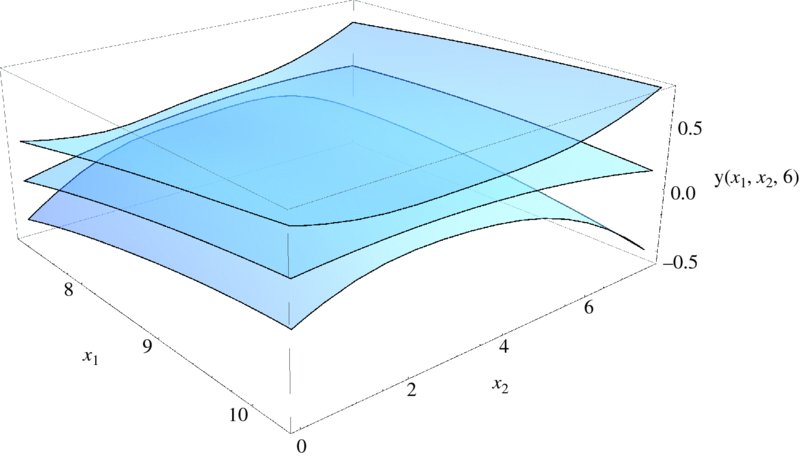
Figure 9.7 Multiple regression fitted surface for x3 = 6 and its confidence interval surfaces
To determine if the residuals are normally distributed, we obtain the probability plot shown in Figure 9.8, by using

Figure 9.8 Normal probability plot of the residuals to the multiple regression fitted surface for x3 = 6
ProbabilityScalePlot[modlm["FitResiduals"],"Normal",
  PlotMarkers->Automatic,
  FrameLabel->{"Residual","Normal Probability"}]
9.4 Nonlinear Regression Analysis: NonLinearModelFit[]
Nonlinear regression analysis is performed with NonLinearModelFit, which is the statistical version of FindFit. FindFit only provides the model’s coefficient, whereas NonLinearModelFit additionally provides several statistical estimates, the same statistical estimates that LinearModelFit provides. The form for NonLinearModelFit is
modl=NonLinearModelFit[coord,{expr,con},par,var,
  ConfidenceLevel->cl]
where coord = {{x1,y1,…,f1},{x2,y2,…,f2},…}, expr is an expression that is a function of the parameters par = {{p1,g1},{p2,g2},…}, where gN are the (optional) guesses for each parameter, var = {x,y,…} are the independent variables, and con are the constraints on the parameters. If there are no constraints, then this quantity is omitted and if no initial guess is provided for a parameter that gM is omitted. The quantity c1 is the confidence level; if omitted, a value of 0.95 is used.
We shall illustrate the use of this function by using the data in Table 5.2 of Exercise 5.33 and assuming that the data can be modeled with the following function

where the constants a, b, c, and d are to be determined. For the initial guess, we shall use a = c = d = 2.0 and b = 0.1 and we shall assume a confidence level of 0.9. The following program will plot the fitted curve, the data values, and the confidence bands as shown in Figure 9.9 and plot the residuals as shown in Figure 9.10. Several of the different entities that can be accessed from the implementation of NonLinearModelFit for this example are summarized in Table 9.8.
Table 9.8 Several output quantities from NonLinearModelFit
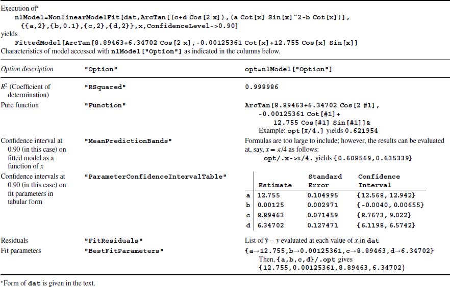

Figure 9.9 Nonlinear curve fit to data values shown and the 90% confidence bands of the fitted curve
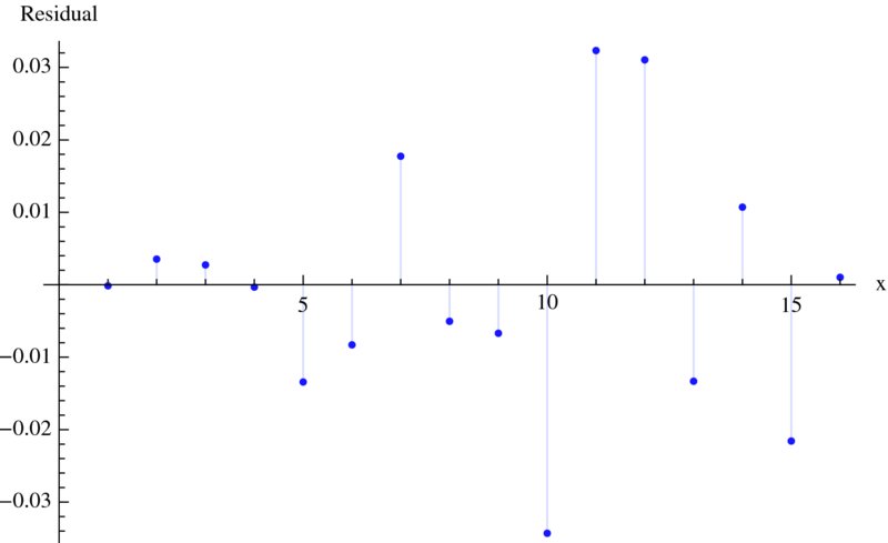
Figure 9.10 Residuals of the nonlinear curve fit given in Figure 9.9
dat={{0.01,0},{0.1141,0.09821},{0.2181,0.1843},
  {0.3222,0.2671},{0.4262,0.3384},{0.5303,0.426},
  {0.6343,0.5316},{0.7384,0.5845},{0.8424,0.6527},
  {0.9465,0.6865},{1.051,0.8015},{1.155,0.8265},
  {1.259,0.7696},{1.363,0.7057},{1.467,0.4338},{1.571,0}};
nlModel=NonlinearModelFit[dat,
  ArcTan[(c+d Cos[2 x]),(a Cot[x] Sin[x]^2-b Cot[x])],
  {{a,2},{b,0.1},{c,2},{d,2}},x,ConfidenceLevel->0.90];
bands=nlModel["MeanPredictionBands"];
Show[Plot[Normal[nlModel],{x,0.01,π/2},
     AxesLabel->{"x","y(x)"}],
  ListPlot[dat,PlotMarkers->Automatic],
  Plot[{bands[[1]],bands[[2]]}/.x->g,{g,0.01,π/2.},
     PlotStyle->{Red,Dashing[Medium]}]]
ListPlot[nlModel["FitResiduals"],Filling->Axis,
  AxesLabel->{"x","Residual"}]
9.5 Analysis of Variance (ANOVA) and Factorial Designs: ANOVA[]
Analysis of variance (ANOVA) is a statistical analysis procedure that can determine whether a change in the output of a process is caused by a change in one or more inputs to the process or is due to a natural (random) variation in the process. In addition, the procedure can also determine if the various inputs to the process interact with each other or if they are independent of each other. The results of ANOVA are typically used to maximize or minimize the output of the process.
Let there be vk, k = 1, 2, …, K inputs to the process and each vk assumes L different values called levels. Each vk, is called a main effect. Each level is identified by an integer that ranges from 1 to L. Corresponding to each level input to the process is the output f. In the physical experiment, the actual values are used to obtain f; however, in the ANOVA analysis the actual values are not used, only the integer designation of its level. We shall designate the value of the input vk at its lth level as lk, where 1 ≤ lj ≤ L. Therefore, the output is f = f(l1, l2,…, lK). When all possible combinations lj are considered, the experiment is considered a full factorial experiment; that is, an analysis where all the main effects and all the interactions of the main effects are considered. In addition, this full combination of levels can be replicated M times so that in general f = f(l1m, l2m,…, lKm), 1 ≤ m ≤ M.
To employ ANOVA, the Analysis of Variance package must first be loaded with
Needs["ANOVA'"]
Then the analysis is performed with
ANOVA[dat,modl,{v1,v2,…,vK}]
where vk, k = 1,2,…,K are the variable names of the main effects, modl is the model to be used, and dat are the data. Using the notation introduced above, the data have the form {{l11,l21,…,lK1,f1},{l12,l22,…lK2,f2},…}, where fn is the value of the output corresponding to the respective combination of levels. For a full factorial experiment, modl is given by {v1,v2,…,vK,All} where All indicates that all combinations of the main effects are to be considered. The effect of All will become clear in the examples that follow.
We shall illustrate the use of ANOVA and the interpretation of the results with the following two examples.
Table 9.9 Data for Example 9.2
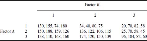
From the ANOVA table, it is seen that the main factors and their interactions are statistically significant at better than the 98% level. Consequently, from an examination of the cell means, if the objective is to find the combination of parameters that produces the maximum output, then one should run the process with factor A at level 2, denoted A[2], and factor B at level 1, denoted B[1]. The output of the process at these levels will be, on average, 155.8. If the interaction term was not statistically significant, then all these interactions would have been ignored; they would be considered a random occurrence. The first value in CellMeans designated All is the overall mean of the data; that is, N[Mean[dat[[All,3]]]] = 105.528.
Table 9.10 Data for Example 9.3

9.6 Functions Introduced in Chapter 9
A list of functions introduced in Chapter 9is given in Table 9.11.
Table 9.11 Commands introduced in Chapter 9
| Command | Usage |
| ANOVA | Performs an analysis of variance |
| BoxWhiskerChart | Creates a box whisker chart |
| CDF | Gives the cumulative distribution function for a specified distribution |
| EstimatedDistribution | Estimates the parameters of a specified distribution for a set of data |
| FindDistributionParameters | Estimates the parameters of a specified distribution for a set of data |
| Histogram | Plots a histogram |
| InverseCDF | Determines the inverse of a specified CDF |
| LinearModelFit | Performs a simple or a multiple linear regression analysis |
| LocationTest | Performs hypothesis tests on means |
| Mean | Obtains the mean of a list of values |
| MeanDifferenceCI | Determines the confidence interval between the means of two lists of values |
| Median | Obtains the median of a list of values |
| NonlinearModelFit | Determines the parameters of a nonlinear model assumed described a list of values |
| NProbability | Determines the probability of an event for a specified probability distribution |
| Gives the symbolic expression or the numerical value of the probability density function for a specified distribution | |
| Probability | Gives the probability of an event for a specified distribution |
| ProbabilityScalePlot | Creates a probability plot of a list of values for a specified distribution |
| Quartile | Give the specified quartile for a list of values |
| RandomVariate | Generates a list of values that have a specified distribution |
| RootMeanSquare | Determines the root mean square of a list of values |
| StudentTCI | Gives the confidence interval of the mean of a list of values |
| StandardDeviation | Obtains the standard deviation of a list of values |
| Variance | Obtains the variance of a list of values |
| VarianceTest | Used to test the hypothesis that the variances of two lists of values are equal |