
10
Control Systems and Signal Processing
10.1 Introduction
A control system is often employed to provide a physical system with the ability to meet specified performance goals. In order to design such a system, one usually creates a model of the physical system and a model of the control system so that the combined system can be analyzed and the appropriate control system characteristics chosen. Mathematica provides a collection of commands that allows one to model the system, analyze the system, and plot the characteristics of the system in different ways. In this chapter, we shall demonstrate the usage of several commands that can be employed to design control systems. In addition, we shall illustrate several commands that can be used in various aspects of signal processing and spectral analysis: filters and windows.
10.2 Model Generation: State-Space and Transfer Function Representation
10.2.1 Introduction
Before illustrating the various Mathematica commands that can be used to represent control systems, we shall introduce a permanent magnet motor as a physical system to be modeled and controlled. This system will be used as the specific linear system when many of the commands are introduced. The governing equations for one such system are [1]
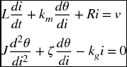
where v = v(t) is the input voltage to the motor windings, i = i(t) is the current in the motor coil, θ = θ(t) is the angular position of the rotor, R is the motor resistance, L is the inductance of the winding, km is the conversion coefficient from current to torque, kg is the back electromotive force generator constant, ζ represents the motor friction, and J is the mass moment of inertia of the system and its load.
10.2.2 State-Space Models: StateSpaceModel[]
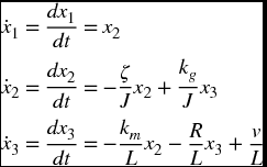
Equation (10.1) can be converted to a system of first-order differential equations with the definitions

Then Eq. (10.1) becomes the following system of first-order equations
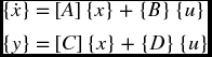
which can be written in matrix form as
where {x} is the state vector, {u} is the input vector, and

The matrix [A] is called the state matrix and the matrix [B] the input matrix.
In addition, we define an output vector {y} as follows
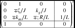
where, for the system under consideration,
It is recalled that x1 = θ. The equations
are the state-space equations for a linear time-invariant system.
The state-space representation for this linear system for the formulation given above is obtained with
StateSpaceModel[{a,b,c,d}]
where a, b, c, and d are the matrices and vectors as defined above. Then, for the system represented by Eq. (10.1),
a={{0,1,0},{0,−ζ/J,kg/J},{0,-km/L,-R/L}};
b={{0},{0},{1/L}};
c={{1,0,0}};
d={{0}};
ssM=StateSpaceModel[{a,b,c,d}]
which displays
The state-space model can also be obtained directly from Eq. (10.1) by using
StateSpaceModel[eqs,x,u,t]
where eqs is a list of the differential equations, x is a list of the dependent variables and their derivatives up to the n − 1 derivative in each dependent variable, u is a list of the input functions, and t is the independent variable. Then, for Eq. (10.1), the state-space equations can be obtained from
StateSpaceModel[{L i’[t]+km θ’[t]+R i[t]==v[t],
   J θ’’[t]+ζθ ’[t]-kg i[t]==0},{θ[t],θ’[t],i[t]},{v[t]},
   {θ[t]},t]
which produces Eq. (10.2).
10.2.3 Transfer Function Models: TransferFunctionModel[]
Equation (10.1) can be converted to a transfer function model by first taking the Laplace transform of these equations assuming zero initial conditions and then solving for the ratio of the Laplace transform of the output variable and the Laplace transform of the input function. Thus, the Laplace transform of Eq. (10.1) with zero initial conditions yields

The solution to Eq. (10.3) is

The transfer function model is created with
TransferFunctionModel[tf,s]
where tf is the transfer function in terms of the variable s. Thus, for the transfer function Θ(s)/V(s) given above,
tfM=TransferFunctionModel[kg/(s ((R+L s) (J s+ζ)+kg km)),s]
which displays

This transfer function representation can also be obtained from the state-space representation obtained previously. In this case, the command argument is
TransferFunctionModel[ssMod]
where ssMod is the state-space model obtained from StateSpaceModel. Thus, for the system under consideration,
Simplify[TransferFunctionModel[ssM]]
creates the same result as that shown in Eq. (10.5).
It is seen that a direct way to arrive at the transfer function is to use the sequence
tfMod=TransferFunctionModel[StateSpaceModel[eqs,x,u,t]]
Thus, for the system given by Eq. (10.1), we have
tfM=TransferFunctionModel[StateSpaceModel[
   {L i’[t]+km θ’[t]+R i[t]==v[t],
      J θ’’[t]+ζ θ’[t]-kg i[t]==0},{θ[t],θ’[t],i[t]},
      {v[t]},{θ[t]},t]]//Simplify
which yields Eq. (10.5).
The transfer function model can be converted to a state-space model with
StateSpaceModel[tfMod]
where tfMod is a transfer function model. Thus, using our previous results,
ssM1=StateSpaceModel[tfM]
displays

which is in a different form than that given by Eq. (10.2) and is a result of the state-space representation not being unique. However, TransferFunctionModel[ssM1] recovers Eq. (10.5).
10.3 Model Connections – Closed-Loop Systems and System Response: SystemsModelFeedbackConnect[] and SystemsModelSeriesConnect[]
There are several commands that allow one to connect transfer function objects to form a closed-loop transfer function model. Two of the most commonly used are as follows. Consider two systems sy1 and sy2 that are transfer function objects. If sy2 is in a feedback loop with sy1, then this system is represented by
SystemsModelFeedbackConnect[sy1,sy2,fbk]
where fbk = −1 is used to indicate negative feedback and fbk = 1 is used for positive feedback. When omitted, the default value is −1. If, in addition, sy2 is omitted, then it is assumed that unity negative feedback is being used.
When these two systems are cascaded, that is, they are in series, then the systems are combined using
SystemsModelSeriesConnect[sy1,sy2]
To illustrate the use of these two commands, we consider the system block diagram shown in Figure 10.1. The transfer function representing the ratio C(s)/R(s) is obtained from
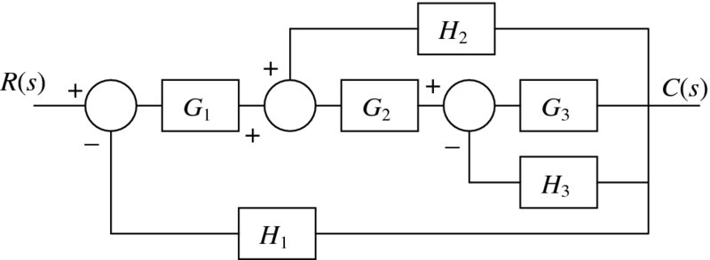
Figure 10.1 Block diagram of interconnected transfer function elements representing a control system
TF[h_]:=TransferFunctionModel[h]
sy1=SystemsModelFeedbackConnect[TF[G3],TF[H3]];
sy2=SystemsModelSeriesConnect[TF[G2],sy1];
sy3=SystemsModelFeedbackConnect[sy2,TF[H2],1];
sy4=SystemsModelSeriesConnect[sy3,TF[G1]];
CR=SystemsModelFeedbackConnect[sy4,TF[H1]]//Simplify
where we have created the function TF to improve the readability of the program. The execution of the program gives
To further illustrate the use of SystemsModelFeedbackConnect, we examine the transfer function given by Eq. (10.5) and make it into a closed-loop system with unity feedback. However, before doing so, we shall introduce a function that can be used to obtain the output response of a system when the input v is specified. The command is
OutputResponse[systfss,v,{t,tmin,tmax}]
when an interpolating function is desired and
OutputResponse[systfss,v,t]
when a symbolic solution function is desired. This symbolic function can be used to determine some of the characteristics of the system’s response such as rise time and percentage overshoot: see Example 10.1.
The system systfss can be either a transfer function model or a state-space model. The state-space model is used when additionally initial conditions are to be specified or initial conditions are specified and v = 0. The quantities tmin and tmax, respectively, indicate the minimum and maximum values of the time interval of interest. The input v is typically DiracDelta to determine the impulse response, UnitStep to determine the response to a step input, and τ−(τ−1) UnitStep[τ−1] to determine the response to a ramp, where τ = t/to and to is the duration of the ramp.
We shall now determine the closed-loop response of the transfer function model given by Eq. (10.5) to a unit step function and display the result. It is assumed that the system has the following parameters: L = 0.01 H, R = 6.0 Ohms, ζ = 0.005 N·m·s·rad−1, km = 0.09 V·s·rad−1, J = 0.02 kg·m2, and kg = 18.0 N·m·A−1. Then,
L=0.01; R=6.; ζ=0.005; km=0.09; J=0.02; kg=18; tend=1.5;
sysnf=TransferFunctionModel[kg/(s ((R+L s) (J s+ζ)+kg km)),s];
tfbk=SystemsModelFeedbackConnect[sysnf[R,L,kg,km,J,ζ]];
sys1out=OutputResponse[tfbk,UnitStep[t],{t,0,tend}];
Plot[sys1out,{t,0,tend},PlotRange->All,
   AxesLabel->{"τ","θ(τ)"}]
which displays the results shown in Figure 10.2.

Figure 10.2 Response to a unit step function of the system given by Eq. (10.5) with unit feedback
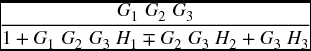
Another useful command for creating stable closed-loop systems is PIDTune. This command allows one to place a general PID controller and any of its special cases in series with a system (denoted sys1) as shown in Figure 10.3. The command automatically selects the parameters of the PID system to reject disturbances and to follow as closely as possible changes in the input signal. The model of this system is given by
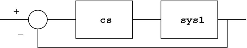
Figure 10.3 Closed-loop system with unity feedback
PIDTune[sys1,{"controller","tuningrule"},"output"]
where sys1 is a transfer function model. The option "controller" is one of several types: "P", "PI", "PID", and a few others. The default controller is "PI". The option "tuningrule" specifies the method that will be used to provide a good estimate of the parameters of the controller that result in stable operation. However, the response may still not satisfy specific transient response characteristics or steady-state characteristics. Therefore, the results from PIDTune may in some cases be a starting point from which one determines the final values of the controller’s parameters. There are 14 tuning rules available; however, not all tuning rules are applicable with all selections of "controller". The default tuning rule is "ZieglerNichols".
The option "output" is used to select one of several output quantities that are available from the function. If this option is omitted, then the transfer function of the "controller" selected is the output. Another output that can be selected is the transfer function of the entire system, which is obtained by using "ReferenceOutput".
Figure 10.4 Response of the control system shown in Figure 10.3 to a unit step input when sys1 is given by Eq. (10.5)
10.4 Design Methods
10.4.1 Root Locus: RootLocusPlot[]
The root locus procedure is used to determine the location of the roots of an open-loop or closed-loop system when a parameter, such as gain, is varied. A plot of the root locus is obtained with
RootLocusPlot[sys,{p,pmin,pmax},PlotPoints->npts,
   PoleZeroMarkers->{Automatic,"ParameterValues"->var}]
where sys is the transfer function of the system, p is the parameter in sys that is to be varied over the range pmin < p < pmax. The option PlotPoints specifies that npts points are to be used to obtain the root locus plot. The option PoleZeroMarkers allows one to place markers at p = var along the locus curves, where var is a single value or a list of values. When one places the cursor over these points, the value of p is shown. By default, Automatic plots a pole with an “×” and a zero with an “![]() ”. The values of these poles and zeros are obtained as indicated subsequently.
”. The values of these poles and zeros are obtained as indicated subsequently.
To illustrate the use of RootLocusPlot, we shall obtain a root locus plot of the closed-loop system shown in Figure 10.3, where cs is now a lead controller whose transfer function is given by
Then, the program that obtains a root locus plot for this system, which is shown in Figure 10.5, is
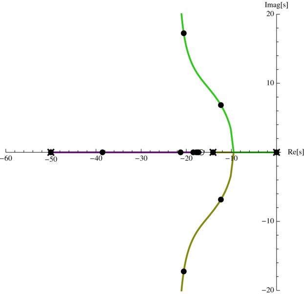
Figure 10.5 Root locus plot of the system shown in Figure 10.3 with cs replaced with the transfer function given by Eq. (10.6)
L=0.01; R=6.; ζ=0.005; km=0.09; J=0.02; kg=18.; tend=1.5;
tf=TransferFunctionModel[kg/(s ((R+L s) (J s+ζ)+kg km)),s];
lead=TransferFunctionModel[ko (3 s+50)/(s+50),s];
sys1=SystemsModelSeriesConnect[lead,tf];
sys=SystemsModelFeedbackConnect[sys1];
RootLocusPlot[sys,{ko,0,15},PlotRange->{{-60,1},{-20,20}},
   PlotPoints->250,AspectRatio->1,
   AxesLabel->{"Re[s]","Imag[s]"},PoleZeroMarkers->
   {Automatic,"ParameterValues"->Range[0,3,0.5]}]
It is mentioned again that when one passes the cursor over the points, the corresponding value of ko is displayed. Also, we have used PlotRange to exclude the most negative pole so that the important part of the root locus plot has ample visual resolution. Setting the aspect ratio to 1 further aids in achieving this visual resolution.
The values of the poles appearing in this figure can be obtained by using
Flatten[TransferFunctionPoles[sys1]]
which yields
{-586.176,-50.,-14.0743,0}
The zeros of the open-loop transfer function are obtained with
Flatten[TransferFunctionZeros[sys1]]
which gives
{-16.6667}
It is shown in the Documentation Center under RootLocusPlot how Manipulate can be used to create an interactive graphic to explore the various aspects of the root locus curves as a function ko.
10.4.2 Bode Plot: BodePlot[]
A Bode plot is a plot of the amplitude in dB of the frequency response of a system and on a separate plot its phase response, usually presented in degrees. A Bode plot is obtained with
BodePlot[sys,StabilityMargins->ft]
where sys is either a transfer function model or a state-space model, and the option StabilityMargins displays on the graph a vertical line indicating the gain and phase margins at the frequencies at which they are determined.
The values of the phase and gain margins can be obtained from
gpm=GainPhaseMargins[sys]
or individually from
gm=GainMargins[sys]
and
gp=PhaseMargins[sys]
In these expressions,
gpm={{{wg1,g1},{wg2,g2},…},{{wp1,p1},{wp2,p2},…}}
gm={{wg1,g1},{wg2,g2},…}
pm={{wp1,p1},{wp2,p2},…}
where wgn is the crossover frequency of the gain margin ratio gn and wpn is the crossover frequency of the phase margin pn in radians.
We shall obtain the Bode plots for the system shown in Figure 10.3 with sys1 given by Eq. (10.5) and cs given by Eq. (10.6) with ko = 3.0 and compare the Bode plots with those in which cs is absent. We shall include the display of the stability margins in the Bode plots and also list their values, which will be converted to dB and degrees. Lastly, we shall display the response of these two systems to a unit step input. Tooltip will also be employed so that placing the cursor over each curve will display the transfer function associated with that curve. The program is
L=0.01; R=6.; ζ=0.005; km=0.09; J=0.02; kg=18.;
ko=3; tend=0.7;
tf=TransferFunctionModel[kg/(s ((R+L s) (J s+ζ)+kg km)),s];
lead=TransferFunctionModel[ko (3s+50)/(s+50),s];
syslead=SystemsModelFeedbackConnect[
   SystemsModelSeriesConnect[lead,tf]];
sysno=SystemsModelFeedbackConnect[tf];
BodePlot[{Tooltip[syslead],Tooltip[sysno]},
   PlotStyle->{{},Dashed}, StabilityMargins->True,
   StabilityMarginsStyle->{{},Dashed}]
orx=OutputResponse[syslead,UnitStep[t],{t,0,tend}];
ory=OutputResponse[sysno,UnitStep[t],{t,0,tend}];
Plot[{orx,ory},{t,0,tend},PlotRange->All,
   AxesLabel->{"t","θ(t)"},
   PlotStyle->{Black,{Black,Dashed}}]
gmlead=GainMargins[syslead];
pmlead=PhaseMargins[syslead];
Map[{#[[1]],#[[2]]/Degree} &,pmlead]
Map[{#[[1]],20.Log10[#[[2]]]} &,gmlead]
which produces the Bode plots shown in Figure 10.6 and the output response to a unit step shown in Figure 10.7. In addition, the program displays the phase margins
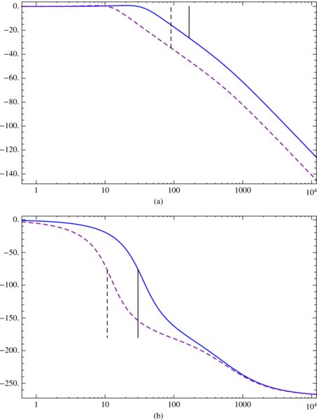
Figure 10.6 Bode plots for the system shown in Figure 10.3 with sys1 given by Eqs. (10.5) and cs given by Eq. (10.6) with ko = 3.0 (solid line) and the Bode plots for the system in which cs is absent (dashed lines): (a) amplitude (b) phase

Figure 10.7 Output responses to a unit step input for the two systems shown in Figure 10.6
{{30.0758,104.239},{0.,180.}}
which are in degrees and the gain margin
{{166.353,26.3221}}
which is expressed in dB.
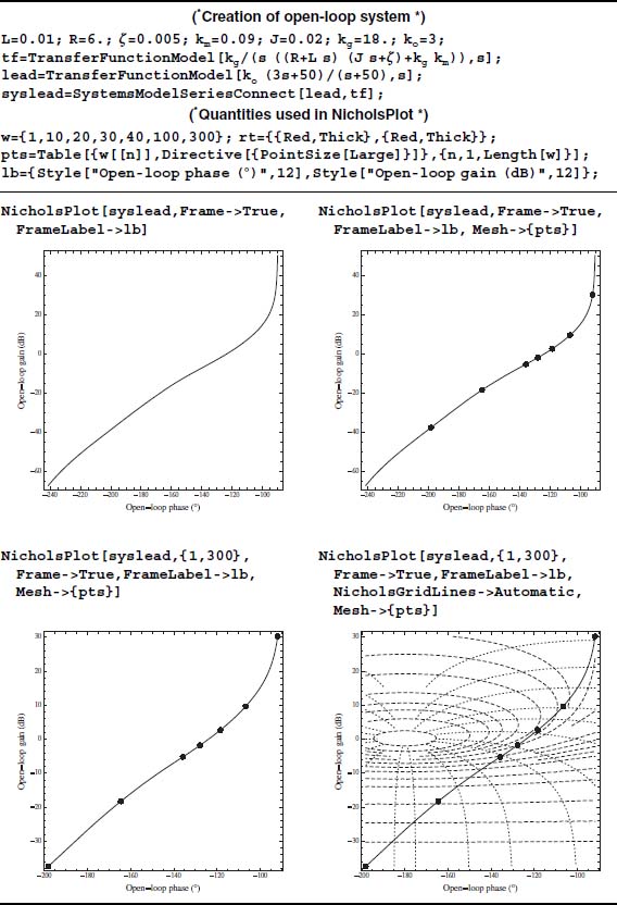
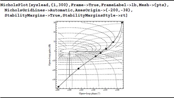
10.4.3 Nichols Plot: NicholsPlot[]
A Nichols plot is a plot of the open-loop or closed-loop system’s phase on the x-axis expressed in degrees versus the open-loop or closed-loop system’s modulus (gain) expressed in dB on the y-axis. It is a very useful tool in frequency-domain analysis. In Mathematica, the creation of a Nichols plot is shown in Table 10.1. As is seen in the table, one must exercise several options to get the plot to look like a classical Nichols chart. It is mentioned that passing the cursor over a grid line displays its value. The values of ω shown as large points on the Nichols curves are as follows: the smallest value of ω in the list w appears at the topmost location and the maximum value of ω at the lowest position. The thick horizontal line emanating from the origin at (−180,0) is the phase margin and the thick vertical line is the corresponding gain margin. Their values can be confirmed with GainMargins and PhaseMargins.
Table 10.1 Creation of a Nichols plot
10.5 Signal Processing
10.5.1 Filter Models: ButterworthFilterModel[], EllipticFilterModel[],…
Mathematica 9 has commands that create the transfer functions of analog filters using different filter models. The models that we shall demonstrate are the Butterworth, elliptic, Chebyshev1, and the Chebyshev2 filters. For each of these models, one can select whether the filter is low pass, high pass, band pass, or band stop. These filter models and types will be examined by displaying the effects that each has on a signal composed of three sinusoidal waves of unit amplitude and different frequencies.
The four commands that create these four transfer functions are defined by the parameters shown in Figure 10.8. In these figures, gs < 1 is the stop-band attenuation, gp ≤ 1 is the pass band attenuation, and gs < gp. The corresponding pass-band frequencies and stop-band frequencies are in rad·s−1.

Figure 10.8 Filter definitions for parameters used in four filter models
The transfer function of a Butterworth filter is obtained with
ButterworthFilterModel[arg]
where arg has one of the following four definitions:
Low-pass filter
{"Lowpass",{wp1,ws1},{ap,as}}
High-pass filter
{"Highpass",{ws1,wp1},{as,ap}}
Band-pass filter
{"Bandpass",{ws1,wp1,wp2,ws2},{as,ap}}
Stop-band filter
{"Bandstop",{wp1,ws1,ws2,wp2},{ap,as}}
In these definitions,
as=-20 Log10[gs]
ap=-20 Log10[gp]
If only a low-pass filter is to be specified, arg is given by {n,wc}, where n is the filter order and wc is the filter’s cutoff frequency.
The remaining filter models can be obtained using
EllipticFilterModel[arg]
Chebyshev1FilterModel[arg]
Chebyshev2FilterModel[arg]
where arg is any one of the four definitions given above.

Figure 10.9 Initial configuration of the interactive graphic to explore the effects of analog filters on sinusoidal signals
10.5.2 Windows: HammingWindow[], HannWindow[],…
In practice, one frequently takes the Fourier transform of signals over a portion of its total duration. This type of transform is called the short-time Fourier transform (STFT). Essentially, one has multiplied the signal by a rectangular window of unit amplitude and duration td. This window is called a Dirichlet window or a rectangular window or a boxcar window and can be represented by the difference of two unit step functions; that is, u(t) − u(t−td). A result of the STFT using the Dirichelt window is to introduce side lobes that sometimes can mask useful information. These side lobes appear when the window does not coincide with the period of a sine wave or a multiple of the periods of a signal with several sine waves. Many window functions have been developed to mitigate this effect. We shall examine, in addition to the rectangular window, five other windows: the Hamming window, the Hann window, the Blackman window, the Kaiser window, and the Nuttall window. The equations that describe each of these functions can be found in the Documentation Center along with about 20 other window functions.1
Before illustrating the window functions, we consider a signal f(t) of duration td composed of two sine waves, one with frequency αfo and unit amplitude and the other with frequency βfo and amplitude A2, where 0.5 ≤ α, β ≤ 2.0, and 0 ≤ A2 ≤ 1. Then,
A window function denoted w(t) is introduced, where w(t) is equal to zero everywhere except for ts ≤ t ≤ ts + tw, ts is the time at which one starts to sample the signal, and tw < td. Then the signal is given by
We are interested in the magnitude of the Fourier transform of Eq. (10.8), which is denoted |Sw(ω)|, where ω is the frequency in rad·s−1. The transform will be obtained with Fourier, which was introduced in Section 5.8. Hence, numerically the signal sw(t) is being sampled every Δt = 1/fs seconds, where for convenience it is assumed that fs = γ fo, where γ > 2. In addition, it is assumed that tw = mγΔt, where m is an integer; thus the sampled function contains nT = mγ samples. It we let ts = nsΔt and t = (ns + n)Δt, where ns is an integer including zero and 1 ≤ n ≤ nT, then the sampled waveform is

Notice that the window function is independent of ns.
The following commands are used to access the selected window functions
wt=DirichletWindow[arg]
wt=HammingWindow[arg]
wt=HannWindow[arg]
wt=BlackmanWindow[arg]
wt=KaiserWindow[arg]
wt=NuttallWindow[arg]
where arg is the independent variable defined over the region −1/2 ≤ arg ≤ 1/2. Therefore, in order to apply these functions to Eq. (10.9), arg is replaced by (n-1)/(nT-1)-1/2, where 1 ≤ n ≤ nT.

Figure 10.10 Initial configuration of the interactive graphic to explore the effects of different windows on two sinusoidal signals
10.5.3 Spectrum Averaging
We shall build on the results of the preceding section and examine the averaging of the spectral content of sinusoidal signals in the presence of noise. Two types of averaging of periodic signals will be considered; root mean square averaging and vector averaging. Root mean square averaging averages the magnitudes of the spectral content on a frequency-by-frequency basis. This type of averaging tends to smooth the spectral magnitudes of the signals of interest, but doesn’t improve the signal-to-noise ratio of the spectrum. For vector averaging, which is also called synchronous averaging, the real parts and imaginary parts of each frequency component are averaged separately. This type of averaging requires a periodically occurring event to trigger the acquisition of the signal. Equation (10.9) is such a signal so that vector averaging can be demonstrated using this signal. This type of averaging can greatly suppress the noise.
The signal that we shall be considering is given by Eq. (10.9), but modified as follows to include additive noise r(t) and account for the kth segment of the signal
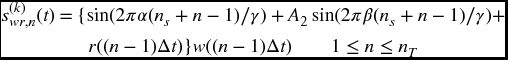
and the superscript k indicates the kth segment of the signal of length nTΔt = nT/(γ fo). We are interested in the manipulation of the components of the Fourier transform of Eq. (10.10) of the kth segment, which are denoted as ![]() , where ωn is the nth discrete frequency in rad·s−1. For root mean square averaging, the magnitude is given by
, where ωn is the nth discrete frequency in rad·s−1. For root mean square averaging, the magnitude is given by
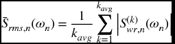
and for vector averaging by

where kavg is the number of segments averaged.
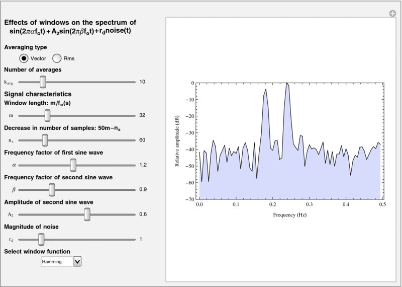
Figure 10.11 Initial configuration of the interactive graphic to explore the effects of different windows and different averaging methods on sinusoidal signals in the presence of noise
10.6 Aliasing
We shall construct an interactive graphic to illustrate aliasing, which is an undesirable consequence of sampling a signal whose highest frequency is fc at an incorrect sampling interval ts; that is, by selecting ts ≥ 1/fs, where fs is the minimum sampling frequency given by fs > αfc. Consider a sine wave of frequency fo such that fo > fc, where fc is used to determine fs. In this case, the signal is being sampled too slowly and as a result the sampled sine wave will appear as a sine wave with aliased frequency fa = fs − fo. In the program, we shall choose fs = αfo, where 1.09 < α < 2.06. In other words, aliasing will occur for α ≤ 2.
If the signal g(t) is uniformly sampled at t = nts, where n is an integer, then the sampled waveform can be recovered from
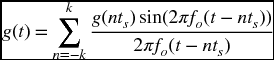
For our purposes, it has been empirically found that

gives good results. This quantity is determined by using Ceiling.

Figure 10.12 Initial configuration of the interactive graphic to illustrate the effects of aliasing
10.7 Functions Introduced in Chapter 10
A list of functions introduced in Chapter 10is given in Table 10.2.
Table 10.2 Commands introduced in Chapter 10
| Command | Usage |
| BlackmanWindow | Represents a Blackman window function |
| BodePlot | Creates a Bode plot from a state-space model or a transfer function model for a time-invariant linear system |
| ButterworthFilterModel | Creates a Butterworth low-pass, high-pass, band-pass, and band-stop filter model |
| Chebyshev1FilterModel | Creates a Chebyshev1 low-pass, high-pass, band-pass, and band-stop filter model |
| Chebyshev2FilterModel | Creates a Chebyshev2 low-pass, high-pass, band-pass, and band-stop filter model |
| DirichletWindow | Represents a Dirichlet (rectangular) window function |
| EllipticFilterModel | Creates an elliptic low-pass, high-pass, band-pass, and band-stop filter model |
| HammingWindow | Represents a Hamming window function |
| HannWindow | Represents a Hann window function |
| KaiserWindow | Represents a Kaiser window function |
| NicholsPlot | Creates a Nichols plot from a state-space model or a transfer function model |
| NuttallWindow | Represents a Nuttall window function |
| OutputResponse | Obtains the numerical output response from a state-space model or a transfer function model for a specified input |
| PIDTune | Creates a PID controller for direct use with a linear time-invariant system |
| RootLocusPlot | Creates a root locus plot from a state-space model or a transfer function model for a time-invariant linear system |
| StateSpaceModel | Creates a standard state-space model or converts a transfer function model to a state-space model |
| SystemsModelFeedbackConnect | Connects the output of system to its input using negative or positive feedback |
| SystemsModelSeriesConnect | Connects two state-space models or two transfer function models in series |
| TransferFunctionModel | Creates a transfer function model or converts a state-space model to a transfer function model |
Reference
- D. K. Anand and R. B. Zmood, Introduction to Control Systems, 3rd edn, Butterworth-Heinemann Ltd. Oxford England, 1995.