1
PROBABILITY
1.1 INTRODUCTION
The theory of probability had its origin in gambling and games of chance. It owes much to the curiosity of gamblers who pestered their friends in the mathematical world with all sorts of questions. Unfortunately this association with gambling contributed to a very slow and sporadic growth of probability theory as a mathematical discipline. The mathematicians of the day took little or no interest in the development of any theory but looked only at the combinatorial reasoning involved in each problem.
The first attempt at some mathematical rigor is credited to Laplace. In his monumental work, Theorie analytique des probabilités (1812), Laplace gave the classical definition of the probability of an event that can occur only in a finite number of ways as the proportion of the number of favorable outcomes to the total number of all possible outcomes, provided that all the outcomes are equally likely. According to this definition, the computation of the probability of events was reduced to combinatorial counting problems. Even in those days, this definition was found inadequate. In addition to being circular and restrictive, it did not answer the question of what probability is,it only gave a practical method of computing the probabilities of some simple events.
An extension of the classical definition of Laplace was used to evaluate the probabilities of sets of events with infinite outcomes. The notion of equal likelihood of certain events played a key role in this development. According to this extension, if Ω is some region with a well-defined measure (length, area, volume, etc.), the probability that a point chosen atrandom lies in a subregion A of Ω is the ratio measure(A)/measure(Ω). Many problems of geometric probability were solved using this extension. The trouble is that one can define “at random” in any way one pleases, and different definitions therefore lead to different answers. Joseph Bertrand, for example, in his book Calcul des probabilités (Paris, 1889) cited a number of problems in geometric probability where the result depended on the method of solution. In Example 9 we will discuss the famous Bertrand paradox and show that in reality there is nothing paradoxical about Bertrand’s paradoxes; once we define “probability spaces” carefully, the paradox is resolved. Nevertheless difficulties encountered in the field of geometric probability have been largely responsible for the slow growth of probability theory and its tardy acceptance by mathematicians as a mathematical discipline.
The mathematical theory of probability, as we know it today, is of comparatively recent origin. It was A. N. Kolmogorov who axiomatized probability in his fundamental work, Foundations of the Theory of Probability (Berlin), in 1933. According to this development, random events are represented by sets and probability is just a normed measure defined on these sets. This measure-theoretic development not only provided a logically consistent foundation for probability theory but also, at the same time, joined it to the mainstream of modern mathematics.
In this book we follow Kolmogorov’s axiomatic development. In Section 1.2 we introduce the notion of a sample space. In Section 1.3 we state Kolmogorov’s axioms of probability and study some simple consequences of these axioms. Section 1.4 is devoted to the computation of probability on finite sample spaces. Section 1.5 deals with conditional probability and Bayes’s rule while Section 1.6 examines the independence of events.
1.2 SAMPLE SPACE
In most branches of knowledge, experiments are a way of life. In probability and statistics, too, we concern ourselves with special types of experiments. Consider the following examples.
The experiments described above have certain common features. For each experiment, we know in advance all possible outcomes, that is, there are no surprises in store after the performance of any experiment. On any performance of the experiment, however, we do not know what the specific outcome will be, that is, there is uncertainty about the outcome on any performance of the experiment. Moreover, the experiment can be repeated under identical conditions. These features describe a random (or a statistical) experiment.
In probability theory we study this uncertainty of a random experiment. It is convenient to associate with each such experiment a set Ω, the set of all possible outcomes of the experiment. To engage in any meaningful discussion about the experiment, we associate with Ω a σ -field ![]() , of subsets of Ω. We recall that a σ -field is a nonempty class of subsets of Ω that is closed under the formation of countable unions and complements and contains the null set Φ.
, of subsets of Ω. We recall that a σ -field is a nonempty class of subsets of Ω that is closed under the formation of countable unions and complements and contains the null set Φ.
The elements of Ω are called sample points. Any set A ∈![]() is known as an event. Clearly A is a collection of sample points. We say that an event A happens if the outcome of the experiment corresponds to a point in A. Each one-point set is known as a simple or an elementary event . If the set C contains only a finite number of points, we say that (Ω,
is known as an event. Clearly A is a collection of sample points. We say that an event A happens if the outcome of the experiment corresponds to a point in A. Each one-point set is known as a simple or an elementary event . If the set C contains only a finite number of points, we say that (Ω, ![]() ) is a finite sample space . If Ωcontains at most a countable number of points, we call (Ω,
) is a finite sample space . If Ωcontains at most a countable number of points, we call (Ω, ![]() ) a discrete sample space. If, however, Ω contains uncountably many points, we say that (Ω,
) a discrete sample space. If, however, Ω contains uncountably many points, we say that (Ω, ![]() )is an uncountable sample space. In particular, if Ω =
)is an uncountable sample space. In particular, if Ω =![]() k or some rectangle in
k or some rectangle in ![]() k , we call it a continuous sample space.
k , we call it a continuous sample space.
Remark 1. The choice of ![]() is an important one, and some remarks are in order. If Ω contains at most a countable number of points, we can always take
is an important one, and some remarks are in order. If Ω contains at most a countable number of points, we can always take ![]() to be the class of all subsets of Ω This is certainly a σ -field. Each one point set is a member of
to be the class of all subsets of Ω This is certainly a σ -field. Each one point set is a member of ![]() and is the fundamental object of interest. Every subset of Ω is an event. If Ω has uncountably many points, the class of all subsets of Ω is still a σ -field, but it is much too large a class of sets to be of interest. It may not be possible to choose the class of all subsets of Ω as
and is the fundamental object of interest. Every subset of Ω is an event. If Ω has uncountably many points, the class of all subsets of Ω is still a σ -field, but it is much too large a class of sets to be of interest. It may not be possible to choose the class of all subsets of Ω as ![]() . One of the most important examples of an uncountable sample space is the case in which Ω=
. One of the most important examples of an uncountable sample space is the case in which Ω=![]() or Ω is an interval in
or Ω is an interval in ![]() . In this case we would like all one-point subsets of Ω and all intervals (closed, open, or semiclosed) to be events. We use our knowledge of analysis to specify
. In this case we would like all one-point subsets of Ω and all intervals (closed, open, or semiclosed) to be events. We use our knowledge of analysis to specify ![]() . We will not go into details here except to recall that the class of all semiclosed intervals (a,b ] generates a class
. We will not go into details here except to recall that the class of all semiclosed intervals (a,b ] generates a class ![]() 1 which is a σ -field on
1 which is a σ -field on ![]() . This class contains all one-point sets and all intervals (finite or infinite). We take
. This class contains all one-point sets and all intervals (finite or infinite). We take ![]() 1. Since we will be dealing mostly with the one-dimensional case, we will write
1. Since we will be dealing mostly with the one-dimensional case, we will write ![]() instead of
instead of ![]() 1. There are many subsets of R that are not in
1. There are many subsets of R that are not in ![]() 1, but we will not demonstrate this fact here. We refer the reader to Halmos
[42]
, Royden
[96]
, or Kolmogorov and Fomin
[54]
for further details.
1, but we will not demonstrate this fact here. We refer the reader to Halmos
[42]
, Royden
[96]
, or Kolmogorov and Fomin
[54]
for further details.


PROBLEMS 1.2
- A club has five members A,B, C, D, and E . It is required to select a chairman and a secretary. Assuming that one member cannot occupy both positions, write the sample space associated with these selections. What is the event that member A is an office holder?
- In each of the following experiments, what is the sample space?
- In a survey of families with three children, the sexes of the children are recorded in increasing order of age.
- The experiment consists of selecting four items from a manufacturer’s output and observing whether or not each item is defective.
- A given book is opened to any page, and the number of misprints is counted.
- Two cards are drawn (i) with replacement and (ii) without replacement from an ordinary deck of cards.
- Let A, B, C be three arbitrary events on a sample space (Ω,
 ). What is the event thatonly A occurs? What is the event that at least two of A, B, C occur? What is the event that both A and C , but not B , occur? What is the event that at most one of A,B,C occurs?
1.3 PROBABILITY AXIOMS
Let (Ω, ![]() )be the sample space associated with a statistical experiment. In this section we define a probability set function and study some of its properties.
)be the sample space associated with a statistical experiment. In this section we define a probability set function and study some of its properties.
In many games of chance, probability is often stated in terms of odds against an event. Thus in horse racing a two dollar bet on a horse to win with odds of 2 to 1 (against) pays approximately six dollars if the horse wins the race. In this case the probability of winningis 1/3.

Fig. 1 A = {(x , y): 0 ≤ x ≤ 1/2, 1/2 ≤ y ≤ 1}.


Fig. 3 C = {(x , y) : (x 2+ y 2 ≤ 1}
Fig. 4 {(x , y) : 0 < x < 1/2 < y < 1, and (y − x) < 1/2 or 0 < y < 1/2 < x < 1, and (x − y) < 1/2}.

Fig. 5 {(x,y): 0 < x <1/2, 1/2 < y <1and 2 (y -x ) <1}.


PROBLEMS 1.3
- Let Ω be the set of all nonnegative integers and S the class of all subsets of Ω. In each of the following cases does P define a probability on (Ω, S)?
- For A , let

- For A , let

- For A ∈
, let PA= 1 if A has a finite number of elements, and PA= 0 otherwise.
- For A
- Let Ω =
 and
and  . In each of the following cases does P define a probability on (Ω, S)?
- For each interval I , let

- For each interval I , let PI= 1if I is an interval of finite length and PI= 0if I is an infinite interval.
- For each interval I , let PI= 0if I ⊆ (-∞,1) and PI = ∫I(1/2) dx if. I ⊆ [1,∞]. (If I = I 1+ I 2, where I 1⊆(-∞,1) and I 2 ⊆ [1,∞), then PI = PI 2.)
- For each interval I , let
- Let A and B be two events such that B⊇A. What is P (A ∪ B) ? What is P (A ∩ B)? What is P (A - B)?
- In Problems 1(a) and (b), let A = {all integers > 2}, B = {all nonnegative integers < 3}, and C = {all integers x , 3 < x < 6}. Find PA , PB , PC , P (A ∩ B), P (A ∪ B), P (B ∪ C), P (A ∩ C), and P (B ∩ C).
- In Problem 2(a) let A be the event A = {x: x ≥0}. Find PA . Also find P {x: x >0}.
- A box contains 1000 light bulbs. The probability that there is at least 1 defective bulb in the box is 0.1, and the probability that there are at least 2 defective bulbs is 0.05. Find the probability in each of the following cases:
- The box contains no defective bulbs.
- The box contains exactly 1 defective bulb.
- The box contains at most 1 defective bulb.
- Two points are chosen at random on a line of unit length. Find the probability that each of the three line segments so formed will have a length > 1/4.
- Find the probability that the sum of two randomly chosen positive numbers (both ≤1) will not exceed 1 and that their product will be ≤2/9.
- Prove Theorem 3.
- Let {An} be a sequence of events such that An→A as n→∞. Show that PAn→PA as n→∞.
- The base and the altitude of a right triangle are obtained by picking points randomly from [0, a] and [0, b], respectively. Show that the probability that the area of the triangle so formed will be less than ab/4 is (1 + ℓn 2)/2.
- A point X is chosen at random on a line segment AB . (i) Show that the probability that the ratio of lengths AX/BX is smaller than a (a > 0) is a/(1 + a). (ii) Show that the probability that the ratio of the length of the shorter segment to that of the larger segment is less than 1/3 is 1/2.
1.4 COMBINATORICS: PROBABILITY ON FINITE SAMPLE SPACES
In this section we restrict attention to sample spaces that have at most a finite number of points. Let Ω = {ω1, ω2,…,ω n}and ![]() be the σ-field of all subsets of Ω. For any A∈
be the σ-field of all subsets of Ω. For any A∈ ![]() ,
,

In games of chance we usually deal with finite sample spaces where uniform probability is assigned to all simple events. The same is the case in sampling schemes. In such instances the computation of the probability of an event A reduces to a combinatorial counting problem. We therefore consider some rules of counting.
Rule 1. Given a collection of n1 elements ![]() elements
elements ![]() and so on, up to nk elements
and so on, up to nk elements ![]() , it is possible to form n 1. n 2..... n k ordered k -tuples
, it is possible to form n 1. n 2..... n k ordered k -tuples ![]() containing one element of each kind, 1
containing one element of each kind, 1 ![]() .
.
PROBLEMS 1.4
- How many different words can be formed by permuting letters of the word “Mississippi”? How many of these start with the letters “Mi”?
- An urn contains R red and W white marbles. Marbles are drawn from the urn one after another without replacement. Let Ak be the event that a red marble is drawn for the first time on the kth draw. Show that
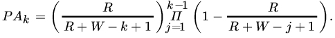
Let p be the proportion of red marbles in the urn before the first draw. Show that
 as
as  . Is this to be expected?
 - In a population of N elements, R are red and W=N-R are white. A group of n elements is selected at random. Find the probability that the group so chosen will contain exactly r red elements.
- Each permutation of the digits 1, 2, 3, 4, 5, 6 determines a six-digit number. If the numbers corresponding to all possible permutations are listed in increasing order of magnitude, find the 319th number on this list.
- The numbers 1, 2 ,…, n are arranged in random order. Find the probability that the digits 1, 2 ,…, k(k<n) appear as neighbors in that order.
- A pin table has seven holes through which a ball can drop. Five balls are played. Assuming that at each play a ball is equally likely to go down any one of the seven holes, find the probability that more than one ball goes down at least one of the holes.
- If 2n boys are divided into two equal subgroups find the probability that the two tallest boys will be (a) in different subgroups and (b) in the same subgroup.
- In a movie theater that can accommodate n + k people, n people are seated. What is the probability that
 given seats are occupied?
- Waiting in line for a Saturday morning movie show are 2 n children. Tickets are priced at a quarter each. Find the probability that nobody will have to wait for change if, before a ticket is sold to the first customer, the cashier has 2 k (k<n) quarters. Assume that it is equally likely that each ticket is paid for with a quarter or a half-dollar coin.
- Each box of a certain brand of breakfast cereal contains a small charm, with k distinct charms forming a set. Assuming that the chance of drawing any particular charm is equal to that of drawing any other charm, show that the probability of finding at least one complete set of charms in a random purchase of
 boxes equals
[ Hint: Use (1.3.6).]
- Prove Rules 1-4.
- In a five-card poker game, find the probability that a hand will have:
- A royal flush (ace, king, queen, jack, and 10 of the same suit).
- A straight flush (five cards in a sequence, all of the same suit; ace is high but A, 2, 3,4, 5 is also a sequence) excluding a royal flush.
- Four of a kind (four cards of the same face value).
- A full house (three cards of the same face value x and two cards of the same face value y).
- A flush (five cards of the same suit excluding cards in a sequence).
- A straight (five cards in a sequence).
- Three of a kind (three cards of the same face value and two cards of different face values).
- Two pairs.
- A single pair.
-
- A married couple and four of their friends enter a row of seats in a concert hall.
What is the probability that the wife will sit next to her husband if all possible seating arrangements are equally likely?
- In part (a), suppose the six people go to a restaurant after the concert and sit at a round table. What is the probability that the wife will sit next to her husband?
- A married couple and four of their friends enter a row of seats in a concert hall.
- Consider a town with N people. A person sends two letters to two separate people, each of whom is asked to repeat the procedure. Thus for each letter received, two letters are sent out to separate persons chosen at random (irrespective of what happened in the past). What is the probability that in the first n stages the person who started the chain letter game will not receive a letter?
- Consider a town with N people. A person tells a rumor to a second person, who in turn repeats it to a third person, and so on. Suppose that at each stage the recipient of the rumor is chosen at random from the remaining N -1 people. What is the probability that the rumor will be repeated n times
- Without being repeated to any person.
- Without being repeated to the originator.
- There were four accidents in a town during a seven-day period. Would you be surprised if all four occurred on the same day? Each of the four occurred on a different day?
- While Rules 1 and 2 of counting deal with ordered samples with or without replacement, Rule 3 concerns unordered sampling without replacement. The most difficult rule of counting deals with unordered with replacement sampling. Show that there are
 possible unordered samples of size r from a population of n elementswhen sampled with replacement.
1.5 CONDITIONAL PROBABILITY AND BAYES THEOREM
So far, we have computed probabilities of events on the assumption that no information was available about the experiment other than the sample space. Sometimes, however, it is known that an event H has happened. How do we use this information in making a statement concerning the outcome of another event A? Consider the following examples.
- Let A and B be two events such that PA=p 1 > 0, PB=p 2 > 0, and p1 + p2 > 1. Show that P {B | A}≥1 − [(1 − p 2) /p 1].
- Two digits are chosen at random without replacement from the set of integers {1, 2, 3, 4, 5, 6, 7, 8}.
- Find the probability that both digits are greater than 5.
- Show that the probability that the sum of the digits will be equal to 5 is the same as the probability that their sum will exceed 13.
- The probability of a family chosen at random having exactly k children is ∝pk ,0 <p< 1. Suppose that the probability that any child has blue eyes is b , 0 <b< 1, independently of others. What is the probability that a family chosen at random has exactly r (r ≥ 0) children with blue eyes?
- In Problem 3 let us write pk = probability of a randomly chosen family having exactly k children = αpk, k = 1,2,…, Suppose that all sex distributions of k children are equally likely. Find the probability that a family has exactly r boys, r ≥ 1. Find the conditional probability that a family has at least two boys, given that it has at least one boy.
- Each of (N + 1) identical urns marked 0, 1, 2,…, N contains N balls. The kth urn contains k black and N –k white balls, k = 0, 1, 2,…, N. An urn is chosen at random, and n random drawings are made from it, the ball drawn being always replaced. If all the n draws result in black balls, find the probability that the (n + 1)th draw will also produce a black ball. How does this probability behave as N →∞?
- Each of n urns contains four white and six black balls, while another urn contains five white and five black balls. An urn is chosen at random from the (n + 1) urns, and two balls are drawn from it, both being black. The probability that five white and three black balls remain in the chosen urn is 1/7. Find n .
- In answering a question on a multiple choice test, a candidate either knows the answer with probability p (0 ≤ p < 1) or does not know the answer with probability 1 – p. If he knows the answer, he puts down the correct answer with probability 0.99, whereas if he guesses, the probability of his putting down the correct result is 1/ k(k choices to the answer). Find the conditional probability that the candidate knew the answer to a question, given that he has made the correct answer. Show that this probability tends to 1 as k→ ∞.
- An urn contains five white and four black balls. Four balls are transferred to a second urn. A ball is then drawn from this urn, and it happens to be black. Find the probability of drawing a white ball from among the remaining three.
- Prove Theorem 2.
- An urn contains r red and g green marbles. A marble is drawn at random and its color noted. Then the marble drawn, together with c > 0 marbles of the same color, are returned to the urn. Suppose n such draws are made from the urn? Find the probability of selecting a red marble at any draw.
- Consider a bicyclist who leaves a point P (see Fig. 1), choosing one of the roads PR1, PR2, PR3 at random. At each subsequent crossroad he again chooses a road at random.
- What is the probability that he will arrive at point A?
- What is the conditional probability that he will arrive at A via road PR 3?
- Five percent of patients suffering from a certain disease are selected to undergo a new treatment that is believed to increase the recovery rate from 30 percent to 50 percent. A person is randomly selected from these patients after the completion of the treatment and is found to have recovered. What is the probability that the patient received the new treatment?

Fig. 1 Map for Problem 11.
- Four roads lead away from the county jail. A prisoner has escaped from the jail and selects a road at random. If road I is selected, the probability of escaping is 1/8; if road II is selected, the probability of success is 1/6; if road III is selected, the probability of escaping is 1/4; and if road IV is selected, the probability of successis 9/10.
- What is the probability that the prisoner will succeed in escaping?
- If the prisoner succeeds, what is the probability that the prisoner escaped by using road IV? Road I?
- A diagnostic test for a certain disease is 95 percent accurate; in that if a person has the disease, it will detect it with a probability of 0.95, and if a person does not have the disease, it will give a negative result with a probability of 0.95. Suppose only 0.5 percent of the population has the disease in question. A person is chosen at random from this population. The test indicates that this person has the disease. What is the (conditional) probability that he or she does have the disease?
1.6 INDEPENDENCE OF EVENTS
Let (Ω, ![]() , P) be a probability space, and let A, B∈
, P) be a probability space, and let A, B∈ ![]() , with PB> 0. By the multiplication rule we have
, with PB> 0. By the multiplication rule we have
In many experiments the information provided by B does not affect the probability of event A, that is, ![]() .
.
We wish to emphasize that independence of events is not to be confused with disjoint or mutually exclusive events. If two events, each with nonzero probability, are mutually exclusive, they are obviously dependent since the occurrence of one will automatically preclude the occurrence of the other. Similarly, if A and B are independent and PA> 0, PB> 0, then A and B cannot be mutually exclusive.
PROBLEMS 1.6
- A biased coin is tossed until a head appears for the first time. Let p be the probability of a head, 0 < p < 1. What is the probability that the number of tosses required is odd? Even?
- Let A and B be two independent events defined on some probability space, and let PA= 1/3, PB= 3/4. Find (a) P(A
 B), (b) P {A | A
  B}, and (c) P {B | A
  B}.
B}. - Let A 1, A 2, and A 3 be three independent events. Show that Ac1,Ac2, and Ac3 are independent.
- A biased coin with probability p,0 < p < 1, of success (heads) is tossed until for the first time the same result occurs three times in succession (i.e., three heads or three tails in succession). Find the probability that the game will end at the seventh throw.
- A box contains 20 black and 30 green balls. One ball at a time is drawn at random, its color is noted, and the ball is then replaced in the box for the next draw.
- Find the probability that the first green ball is drawn on the fourth draw.
- Find the probability that the third and fourth green balls are drawn on the sixth and ninth draws, respectively.
- Let N be the trial at which the fifth green ball is drawn. Find the probability that the fifth green ball is drawn on the n th draw. (Note that N take values 5, 6, 7, …)
- An urn contains four red and four black balls. A sample of two balls is drawn at random. If both balls drawn are of the same color, these balls are set aside and a new sample is drawn. If the two balls drawn are of different colors, they are returned to the urn and another sample is drawn. Assume that the draws are independent and that the same sampling plan is pursued at each stage until all balls are drawn.
- Find the probability that at least n samples are drawn before two balls of the same color appear.
- Find the probability that after the first two samples are drawn four balls are left, two black and two red.
- Let A , B , and C be three boxes with three, four, and five cells, respectively. There are three yellow balls numbered 1 to 3, four green balls numbered 1 to 4, and five red balls numbered 1 to 5. The yellow balls are placed at random in box A, the green in B, and the red in C, with no cell receiving more than one ball. Find the probability that only one of the boxes will show no matches.
- A pond contains red and golden fish. There are 3000 red and 7000 golden fish, of which 200 and 500, respectively, are tagged. Find the probability that a random sample of 100 red and 200 golden fish will show 15 and 20 tagged fish, respectively.
- Let (Ω, , P)be a probability space. Let A, B, C∈ with PB and PC> 0. If B and C are independent show that

Conversely, if this relation holds, P{A I BC} ≠ P{A I B}, and PA> 0, then B and C are independent (Strait [111] ).
- Show that the converse of Theorem 2 also holds. Thus A and B are independent if, and only if, A and Bc are independent, and so on.
- A lot of five identical batteries is life tested. The probability assignment is assumed to be

for any event A ⊆[0,∞ ), where λ> 0 is a known constant. Thus the probability that a battery fails after time t is given by

If the times to failure of the batteries are independent, what is the probability that at least one battery will be operating after t 0hours?
- On Ω = (a, b) , −∞<a<b< ∞, each subinterval is assigned a probability proportional to the length of the interval. Find a necessary and sufficient condition for two events to be independent.
- A game of craps is played with a pair of fair dice as follows. A player rolls the dice. If a sum of 7 or 11 shows up, the player wins; if a sum of 2, 3, or 12 shows up, the player loses. Otherwise the player continues to roll the pair of dice until the sum is either 7 or the first number rolled. In the former case the player loses and in the latter the player wins.
- Find the probability that the player wins on the n th roll.
- Find the probability that the player wins the game.
- What is the probability that the game ends on: (i) the first roll, (ii) second roll, and (iii) third roll?