Dose-Response Safety Analyses Using Large Health Care Databases
13.3 Treatment Model and Censoring Model Setup
13.4 Structural Model Implementation
The marginal structural models (MSM) method has been introduced in Chapter 9 in a traditional two-group comparison setting. In this chapter, the application of MSM is demonstrated using a large observational database to assess dose response of a single treatment that’s dynamic over time. The endpoint is mortality, which frequently is the focus of analyses performed using such databases.
13.1.1 Overview
While clinical trials in a controlled environment provide the basis for regulatory approval, large-scale observational databases are usually the means for long-term safety assessment. Statistical methods are critical in dealing with such databases because the data almost without exception suffer from confounding, sometimes even time-dependent confounding. In this chapter the marginal structural models (MSMs) approach is illustrated in analyzing safety information using such a database. It uses inverse probability of treatment weights to create a pseudo-randomized population to facilitate causal inferences. The association between treatments and safety signals is less confounded and, under the assumption of no model misspecification, may even have a causal interpretation. The approach is demonstrated using a dialysis claims database to study the Epoetin alfa dose relationship with mortality. This large-scale database contains additional variables that are not often found in smaller databases, and through the MSM analysis, these additional variables enabled us to reduce the impact of confounding and to more precisely estimate the hazard ratios associated with treatment dosage.
We first introduce some background information on the complex and dynamic interactions among end-stage renal disease (ESRD), anemia, and dialysis treatment, together with some conventional analyses that attempt to assess the dose-mortality relationship. The fact that these analyses suffer from apparent confounding makes it clear that more sophisticated causal inference methods should be applied. Next, we describe in detail the database used and its structure that facilitates the MSM analysis. Following the technical details presented in Chapter 9, we then describe the setup of the treatment model, the censoring model, and the structural model that we used to carry out the MSM analysis. SAS code and the main SAS output are included. Results are interpreted based on these outputs, and some discussions are provided on the caveats in performing analysis using MSM.
13.1.2 Disease, Treatment, and Analysis Background
Patients who suffer from kidney failure almost always experience anemia as a co-morbid condition. This is because erythropoietin, a protein that regulates red blood cell production, is produced in the kidney. End-stage renal disease results in decreased production of erythropoietin by the kidneys, which then causes low levels of hemoglobin, or anemia. Dialysis treatment helps maintain the body’s internal equilibrium of water and minerals, but it does not compensate for the lost erythropoietin function. Therefore, an important aspect of dialysis treatment is anemia management. Over the years, the standard of care in the dialysis setting has evolved to routinely include erythropoiesis-stimulating agents, or ESAs. ESAs are proteins that function as endogenous erythropoietin but are manufactured using recombinant DNA technology. The clinical benefit of ESAs is to increase the red blood cell level, measured by hemoglobin (Hb, in g/dL). An ESA that has been used since the early 1990’s is Epoetin alfa (Epogen, Amgen Inc., Thousand Oaks, CA).
Some analyses based on observational data have attempted to assess the safety outcomes of Epoetin alfa. The most noticeable analysis involved association between Epoetin alfa dose and mortality using conventional Cox model, with dose as a baseline or time-dependent variable. For example, the analysis conducted by Zhang and colleagues (2004) seemed to show a clear trend of higher mortality associated with higher dose. This finding was replicated using the same statistical method by Bradbury and colleagues (2008) (Figure 13.1). Using a more granular data set, Bradbury and colleagues (2008) showed that the hazard ratio (HR) was approximately 1.22 using dose at baseline, and it dropped to around 1.0 when dose was used as a time-dependent variable.
Figure 13.1 Conventional Cox Regression Results
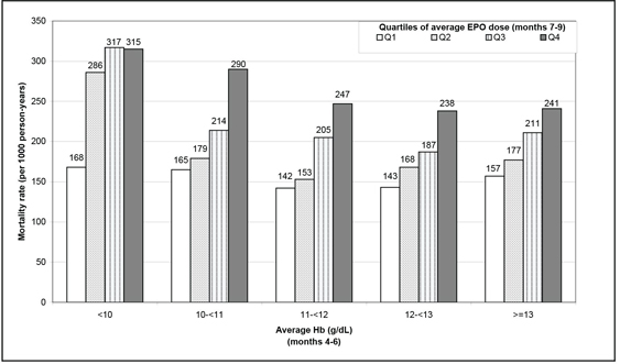
However, it is well recognized that sicker patients have lower Hb levels and are likely to be prescribed higher doses of Epoetin alfa. The sicker patients also are more likely to die. This is a classic confounding problem for point treatment cases. Moreover, observed Hb levels affect subsequent Epoetin alfa dose prescription, which in turn impacts the following Hb level. In order to maintain a certain Hb level, Epoetin alfa doses need to be adjusted periodically. Therefore, it’s a typical time-dependent confounding problem. As mentioned in Chapter 9, traditional inferences in this situation, including Cox proportional hazard models with time-dependent treatment, do not have a causal interpretation. This is because the assumptions required for a causal interpretation do not hold due to the presence of confounding. In order to assess the causal relationship between Epoetin alfa doses and mortality, more sophisticated statistical methods are called for, and we used a marginal structural model as an alternative (Robins et al., 2000; Hernán et al., 2000).
We have obtained medical records data from one of the dialysis chains. A subset of patient data collected by this dialysis chain is available to us under private utilization agreements. These data include patient demographics, ESA doses, Hb levels, and co-morbid conditions. Numerous analyses have been done using data from dialysis chains to understand treatment effects and improve patient care.
Note that another example demonstrating the MSM application is discussed in Chapter 9. However, this chapter is different because the outcome here is survival. We discuss a single treatment at different doses instead of two treatment groups, and dose response is our focus rather than a comparison between two treatment groups.
Before we dive into the MSM analysis details, let’s first understand the database at hand. This dialysis chain provides hemodialysis to more than 100,000 patients in the United States and collects information on laboratory parameters, medications, demographic characteristics, dialysis care, and clinical outcomes, including hospitalization and death. For this analysis, data were available for a random sample of 60,000 hemodialysis patients who were at least 18 years of age with no history of peritoneal dialysis and who received hemodialysis for at least 1 month between July 2000 and June 2002. We restricted our study population to patients whose first appearance in the database was before January 2001 and who had a 6-month baseline period to allow for patient characterization. Patients were followed up for 12 months.
Most laboratory parameters (for example, albumin, ferritin, transferrin saturation [TSAT]) were collected monthly; hemoglobin values were collected more frequently (about two times per month) in most facilities. Data were available for Epoetin alfa (EPO) and iron doses (recorded at each administration), demographic characteristics (captured when patients began receiving dialysis), and dialysis care information, including urea reduction ratio (URR), number of missed dialysis visits, and vascular access (VA) information. Hospitalization data were collected on an ongoing basis and included admission and discharge dates and diagnoses based on International Classification of Disease—9th Revision (ICD-9) codes. Mortality information was routinely collected, as were reasons for loss to follow up, which included renal transplantation, facility transfer, withdrawal, and modality change.
We assessed Epoetin alfa dosing at 2-week intervals, to be consistent with the Hb assessment frequency in usual care. In each interval, we calculated the cumulative outpatient Epoetin alfa dose (sum of all available doses recorded in the dialysis facility). Epoetin alfa dosing information is not captured in the inpatient setting and, therefore, was unavailable to us. For the purpose of this analysis, we imputed the inpatient portion of the Epoetin alfa treatment using the last dose before hospitalization.
The reason that this database was selected for this analysis, as opposed to other choices (for example, the United States Renal Data System [USRDS] data collected through Medicare), is that Epoetin alfa dose information is available for every administration, and all assessed Hb values are available in the database. In other words, the critical data are much more granular than databases used in other analyses; that is, the data include more observations of more variables and, in general, provide a more complete view of the patient condition, treatment factors, and variables used by doctors in making dosing decisions. This should be an important consideration when applying the MSM analysis because the assumption of no unmeasured confounders is a critical assumption for causal inferences.
The actual SAS database used in this analysis has one record per patient-time point. Patient characteristics were assessed through a corresponding demographics database (with one record per patient) using Program 13.1 to provide a general idea of the patient population. The SAS output is quite long and, instead of the SAS output display, the results are summarized in Table 13.1 as a more concise alternative. Continuous variables are presented as mean (standard deviation) and categorical variables as count (frequency). Note that the summaries are presented per dose categories (bldosequartile, or baseline dose quartiles, plus the zero dose group), which is explained in more detail later.
Program 13.1 Patient Characteristics Summary
*** Compute means for continuous variables;
proc means data=demog mean;
var AGE HEMODIALYRS BMI BLFER BLSAT BLALB BLHGB;
by bldosequartile;
OUTPUT OUT=mean MEAN=AGE HEMODIALYRS BMI BLFER BLSAT BLALB BLHGB;
run;
*** Compute standard deviations for continuous variables;
proc means data=demog stddev;
var age HEMODIALYRS BMI BLFER BLSAT BLALB BLHGB;
by bldosequartile;
OUTPUT out=stddev stddev=AGE HEMODIALYRS BMI BLFER BLSAT BLALB BLHGB;
run;
*** Compute count and frequency for categorical variables;
proc freq data=demog;
table AGEGROUP/out=a;
table ETH/out=b;
table SEX/out=c;
table REGION/out=d;
table BLHYPERTENSN/out=e;
table GLE/out=f;
by bldosequartile;
run;
Similar code was run for the overall patient population.
Table 13.1 Patient Demographics and Baseline Characteristics
| Dose group 0 | Dose group 1 | Dose group 2 | Dose group 3 | Dose group 4 | All | |
| N | 304 | 5544 | 7904 | 8336 | 5703 | 27791 |
| Age (years) | 54.77 (13.99) | 61.01 (15.01) | 61.8 (15.08) | 60.51 (14.73) | 58.13 (14.74) | 60.43 (14.74) |
| Dialysis Vintage (years) | 4.95 (4.77) | 3.44 (3.81) | 2.66 (3.28) | 2.49 (3.36) | 2.83 (3.6) | 2.82 (3.6) |
| Baseline BMI (kg/m2) | 27.98 (8.07) | 26.17 (6.69) | 26.37 (6.65) | 27.17 (7.15) | 28.27 (7.9) | 26.98 (7.9) |
| Baseline Ferritin (ng/ml) | 500.8 (322.9) | 591.8 (360.7) | 527.4 (341.5) | 478.7 (343.6) | 473.3 (351.8) | 514.2 (351.8) |
| Baseline TSAT (%) | 31.54 (10.44) | 32.08 (9.66) | 29.12 (9.17) | 26.49 (8.88) | 24.32 (9.33) | 27.97 (9.33) |
| Baseline Albumin (g/dl) | 3.88 (0.32) | 3.89 (0.28) | 3.83 (0.3) | 3.76 (0.33) | 3.66 (0.36) | 3.79 (0.36) |
| Baseline Hb (g/dl) | 12.9 (1.31) | 12.11 (0.78) | 11.89 (0.76) | 11.63 (0.88) | 11.01 (1.07) | 11.69 (1.07) |
| Age < 45 years | 83 (27.3) | 831 (15) | 1159 (14.7) | 1304 (15.6) | 1103 (19.3) | 4480 (16.1) |
| Age >= 45 to < 65 years | 138 (45.4) | 2181 (39.3) | 2869 (36.3) | 3304 (39.6) | 2482 (43.5) | 10974 (39.5) |
| Age >= 65 years | 83 (27.3) | 2532 (45.7) | 3876 (49) | 3728 (44.7) | 2118 (37.1) | 12337 (44.4) |
| Female | 83 (27.3) | 2252 (40.6) | 3835 (48.5) | 4197 (50.3) | 2908 (51) | 13275 (47.8) |
| Black | 128 (42.1) | 2060 (37.2) | 3030 (38.3) | 3548 (42.6) | 2778 (48.7) | 11544 (41.5) |
| Region=MIDWEST | 39 (12.8) | 488 (8.8) | 758 (9.6) | 841 (10.1) | 568 (10) | 2694 (9.7) |
| Region=NORTHEAST | 50 (16.4) | 927 (16.7) | 1277 (16.2) | 1450 (17.4) | 1111 (19.5) | 4815 (17.3) |
| Region=SOUTH | 184 (60.5) | 3226 (58.2) | 4847 (61.3) | 5265 (63.2) | 3595 (63) | 17117 (61.6) |
| Region=WEST | 31 (10.2) | 903 (16.3) | 1022 (12.9) | 780 (9.4) | 429 (7.5) | 3165 (11.4) |
| Hypertension | 42 (13.8) | 729 (13.1) | 1170 (14.8) | 1343 (16.1) | 997 (17.5) | 4281 (15.4) |
| Diabetic | 116 (38.2) | 2630 (47.4) | 4087 (51.7) | 4446 (53.3) | 2875 (50.4) | 14154 (50.9) |
13.3 Treatment Model and Censoring Model Setup
We estimated the mortality hazard ratio using marginal structural models (MSMs), where the inverse probability of treatment weighting (IPTW) was used to adjust for confounding by indication. This two-step approach calculates the weights first as the inverse of the predicted Epoetin alfa doses using a treatment model and then assesses the HRs using a weighted structural model. Specifically, IPTW down-weights patients who receive doses close to what was predicted and up-weights patients who receive doses that vary appreciably from what was predicted. This weighting creates a pseudo-population in which confounding between factors influencing treatment and the actual treatment received is mitigated. Consequently, HRs based on this pseudo-population can have a causal interpretation, provided that the weights are modeled accurately and other assumptions are met (Robins, 2000). One important assumption is the ETA assumption—namely, the probability of observing a specific treatment regimen is >0 and <1. In other words, the treatment decision is not a deterministic function of the past. Therefore, each treatment decision is not independent and random (otherwise there is no confounding) and yet cannot be fixed given the past either.
We calculated treatment weights, which were related to predicted EPO doses, for each patient in 2-week intervals using ordinal regression. Our goal was to construct a model that reflects the physician decision-making process in deciding what the next Epoetin alfa dose is for a particular patient. The model is constructed using the entire patient population, and both statistical and clinical considerations are put to work. A simple approach is to recognize the role of observed Hb values and the inertia/momentum of previous doses. This results in a “simple” model with Hb and dose in the previous four time intervals. Some clinicians argue that they also take into consideration a patient’s hospitalization status, iron indices, vascular access, and other co-morbid conditions. That led to an “expanded” model, which added days in hospital, number of non-hospital doses, albumin, ferritin, TSAT, vascular access type, hypertension status, and dialysis adequacy in the previous time interval to the simple model. Finally, a “full” model was constructed by adding the interaction between Hb and dose to the “expanded” model, recognizing the dynamics between the two factors, which makes good clinical sense.
The calculations are implemented in SAS using PROC GENMOD. The three models are implemented similarly, and only the full model is illustrated here. Note that the treatment weights are ratios, with the time-dependent confounders included in the denominator only. See Program 13.2. The numerator and the denominator, both predicted dose quartiles, are calculated separately. Weights calculated this way are called stabilized weights, denoted as “sw”.
Program 13.2 Treatment Weights Calculation
*** Compute the treatment part of the IPTW weights;
*** Numerator part, including baseline covariates and time-dependent intercept;
proc genmod data=infile rorder=formatted order=formatted;
class ETH SEX REGION VITDFLAG GLU BLVAC CDAYSINHOSP BLHYPERTENSN
BLHXADEQUACY bldosequartile lag1dosequartile lag2dosequartile
lag3dosequartile lag4dosequartile
lag1HYPERTENSION lag1HXADEQUACY lag1VASCULAR;
model dosequartile = ETH SEX REGION VITDFLAG GLU BLVAC
CDAYSINHOSP BLHYPERTENSN BLHXADEQUACY AGE BMI HEMODIALYRS
NOCHGDOSES NOHLDDOSES PERLESS11 BLHGB BLIRON BLALB BLFER BLSAT
BLPTH bldosequartile lag1dosequartile lag2dosequartile
lag3dosequartile lag4dosequartile
hmthno hmthno1 hmthno2 hmthno3
/ dist=multinomial link=clogit;
output out=preds pred=pred;
run;
proc sort data=preds;
by patient biweekno dosequartile _order_;
run;
proc transpose data=preds out=predst(keep=patient theta1 theta2 theta3
theta4 biweekno dosequartile) prefix=theta;
by patient biweekno dosequartile;
id _order_;
var pred;
run;
data model1;
set predst;
prob1=theta1;
prob2=theta2-theta1;
prob3=theta3-theta2;
prob4=theta4-theta3;
prob5=1-theta4;
if dosequartile=1 then treat_top=prob1;
else if dosequartile=2 then treat_top=prob2;
else if dosequartile=3 then treat_top=prob3;
else if dosequartile=4 then treat_top=prob4;
else if dosequartile=5 then treat_top=prob5;
keep patient biweekno dosequartile treat_top;
run;
*** Denominator part, including baseline covariates, time-dependent intercept, and also any time-dependent covariates;
proc genmod data=infile rorder=formatted order=formatted;
class ETH SEX REGION VITDFLAG GLU BLVAC CDAYSINHOSP BLHYPERTENSN
BLHXADEQUACY bldosequartile lag1dosequartile lag2dosequartile
lag3dosequartile lag4dosequartile
lag1HYPERTENSION lag1HXADEQUACY lag1VASCULAR;
model dosequartile = ETH SEX REGION VITDFLAG GLU BLVAC
CDAYSINHOSP BLHYPERTENSN BLHXADEQUACY AGE BMI HEMODIALYRS
NOCHGDOSES NOHLDDOSES PERLESS11 BLHGB BLIRON BLALB BLFER BLSAT
BLPTH bldosequartile lag1dosequartile lag2dosequartile
lag3dosequartile lag4dosequartile
lag1hb lag2hb lag3hb lag4hb
lag1HYPERTENSION lag1HXADEQUACY lag1VASCULAR lag1NHSPDNUM
lag1hospitaldays lag1iron lag1sat lag1alb lag1fer
lag1hbdose0 lag1hbdose1 lag1hbdose2 lag1hbdose3 lag1hbdose4
hmthno hmthno1 hmthno2 hmthno3
/ dist=multinomial link=clogit;
output out=preds pred=pred;
run;
proc sort data=preds;
by patient biweekno dosequartile _order_;
run;
proc transpose data=preds out=predst(keep=patient theta1 theta2 theta3
theta4 biweekno dosequartile) prefix=theta;
by patient biweekno dosequartile;
id _order_;
var pred;
run;
data model2;
set predst;
prob1=theta1;
prob2=theta2-theta1;
prob3=theta3-theta2;
prob4=theta4-theta3;
prob5=1-theta4;
if dosequartile=1 then treat_bottom=prob1;
else if dosequartile=2 then treat_bottom=prob2;
else if dosequartile=3 then treat_bottom=prob3;
else if dosequartile=4 then treat_bottom=prob4;
else if dosequartile=5 then treat_bottom=prob5;
keep patient biweekno dosequartile treat_top;
run;
data trtmodels;
merge model1 (keep=patient biweekno treat_top)
model2 (keep=patient biweekno treat_bottom)
by patient biweekno;
if nmiss(treat_top, treat_bottom)>0 then treat_sw=1;
if nmiss(treat_top, treat_bottom)=0 then
treat_sw=treat_top/treat_bottom;
run;
In a usual MSM implementation, weights at each time point are aggregated by multiplying all the weights in the study prior to the particular time point. As can be imagined, the variability associated with weights at later time points gets bigger and bigger. These weights are summarized and illustrated in Figure 13.2.
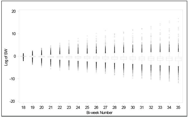
In complicated treatment scenarios with a titratable drug, some of the calculated IPTWs could get very large due to unusual patient characteristics, unconventional treatment decisions, large variability in data assessment, or even data recording errors. Model inadequacy early on may cause the inaccurate weights to be multiplied again and again for later time points because weights are cumulative. In order to prevent the analysis from being dominated by a handful of patients with large weights, in our implementation of MSM the aggregated weights were calculated based on only the previous four time intervals, instead of all previous time points. This variation has the effect of stabilizing the weights, as shown in Figure 13.3. Note the smaller range and the uniformity of the range over the bi-weekly periods. We also truncated the highest weight to either the 98th or 99th percentile values (weights of 82 and 471, respectively, in the full treatment model case). By excluding relatively few outliers that would otherwise greatly influence the model, we were able to improve the performance of the hazard ratio estimates using MSM.
Figure 13.3 Modified MSM Weights

Patient censoring was considered in a similar way to the treatment information, predicted at each time point (given the observed past), and incorporated into the weighting. Censoring events included loss to follow up for various reasons. Censoring weights are calculated using Program 13.3, which is similar to Program 13.2. The censoring weights are not summarized here.
Program 13.3 Censoring Weights Calculation
*** Compute the censoring part of the IPTW weights;
*** Numerator part, including baseline covariates and time-dependent intercept;
proc logistic data=infile;
class lag1dosequartile lag2dosequartile lag3dosequartile
lag4dosequartile bldosequartile ETH SEX REGION VITDFLAG GLU BLVAC
CDAYSINHOSP BLHYPERTENSN BLHXADEQUACY;
model censored = lag1dosequartile lag2dosequartile
lag3dosequartile lag4dosequartile bldosequartile ETH SEX REGION
VITDFLAG GLU BLVAC DAYSINHOSP BLHYPERTENSN BLHXADEQUACY AGE BMI
HEMODIALYRS NOCHGDOSES NOHLDDOSES PERLESS11 BLHGB BLIRON BLALB
BLFER BLSAT BLPTH hmthno hmthno1 hmthno2 hmthno3;
output out=model3 p=censored_top;
run;
*** Denominator part, including baseline covariates, time-dependent intercept, and also any time-dependent covariates;
proc logistic data=infile;
class ETH SEX REGION VITDFLAG GLU BLVAC CDAYSINHOSP BLHYPERTENSN
BLHXADEQUACY bldosequartile
lag1dosequartile lag2dosequartile lag3dosequartile lag4dosequartile
lag1HYPERTENSION lag1HXADEQUACY lag1VASCULAR;
model censored = ETH SEX REGION VITDFLAG GLU BLVAC CDAYSINHOSP
BLHYPERTENSN BLHXADEQUACY AGE BMI HEMODIALYRS
NOCHGDOSES NOHLDDOSES PERLESS11 BLHGB BLIRON BLALB BLFER BLSAT BLPTH
bldosequartile lag1dosequartile lag2dosequartile lag3dosequartile lag4dosequartile
lag1hb lag2hb lag3hb lag4hb
lag1HYPERTENSION lag1HXADEQUACY lag1VASCULAR lag1NHSPDNUM
lag1hospitaldays lag1iron lag1sat lag1alb lag1fer
lag1hbdose0 lag1hbdose1 lag1hbdose2 lag1hbdose3 lag1hbdose4 hmthno
hmthno1 hmthno2 hmthno3;
output out=model4 p=censored_bottom;
run;
data censormodels;
merge model3 (keep=patient biweekno censored_top)
model4 (keep=patient biweekno censored_bottom) ;
by patient biweekno;
if nmiss(censored_top, censored_bottom)>0 then censored_sw=1;
if nmiss(censored_top, censored_bottom)=0 then
censored_sw=censored_top/censored_bottom;
run;
13.4 Structural Model Implementation
The structural model is step two in the MSM method implementation. This is where the causal inferences are made using weighted observations. In our database, the clinical outcome we are assessing is mortality, and survival analysis is needed to estimate its relationship with dose. The actual implementation in SAS, however, is through PROC GENMOD because PROC PHREG does not handle weighted analyses. The generalized estimating equations (GEE) approach using PROC GENMOD is used for hazard ratio point estimates. The confidence intervals associated with these point estimates must be derived from bootstrapping instead of directly utilizing intervals produced by PROC GENMOD. This is discussed in detail later.
The GEE model includes dose and baseline covariates to estimate mortality hazard ratios, with weighting on the Epoetin alfa doses. Mortality was assessed during a 1-year period following the patient’s index date and aggregated into bi-weekly intervals. Epoetin alfa doses were grouped into a zero dose category and dose quartiles (1st quartile: ≤ 14000 IU/2 weeks; 2nd quartile: 14000–27000 IU/2 weeks; 3rd quartile: 27000–49000 IU/2 weeks; 4th quartile: > 49000 IU/2 weeks). The lowest non-zero dose quartile was used as the reference group in the structural model. The exposure variable, Epoetin alfa dose category, was lagged by 8 weeks (four time intervals) to allow for the fact that severely ill patients are often hospitalized approximately 4 to 8 weeks prior to death, and their in-hospital Epoetin alfa doses, if any, were not available in our database, which was collected through the dialysis chain. For patients with missed Epoetin alfa doses or patients who did not receive a dose during a dialysis session, a zero dose was recorded. For patients who survived hospitalization, an in-hospital Epoetin alfa dose was imputed using the most recent dose prior to hospitalization.
Program 13.4 implements the structural model using GEE.
proc genmod data=allmodels descending;
class patient ETH SEX REGION VITDFLAG GLU BLVAC CDAYSINHOSP
BLHYPERTENSN BLHXADEQUACY bldosequartile;
model die = ETH SEX REGION VITDFLAG GLU BLVAC CDAYSINHOSP
BLHYPERTENSN BLHXADEQUACY AGE BMI HEMODIALYRS NOCHGDOSES
NOHLDDOSES PERLESS11 BLHGB BLIRON BLALB BLFER BLSAT BLPTH
bldosequartile epoq0 epoq2 epoq3 epoq4
hmthno hmthno1 hmthno2 hmthno3
/link=logit dist=bin;
scwgt wgt;
repeated subject=patient/type=ind;
run;
Output from Program 13.4
Analysis Of GEE Parameter Estimates
Empirical Standard Error Estimates
| Parameter | Estimate | Standard Error | 95% Confidence Limits |
Z Pr > |Z| | |||
| Intercept | 0.7441 | 2.1078 | -3.3871 | 4.8753 | 0.35 | 0.7241 | |
| Eth | 0 | 0.3070 | 0.0853 | 0.1398 | 0.4743 | 3.60 | 0.0003 |
| Eth | 1 | 0.0000 | 0.0000 | 0.0000 | 0.0000 | ||
| Sex | 0 | -0.1429 | 0.0625 | -0.2653 | -0.0205 | -2.29 | 0.0221 |
| Sex | 1 | 0.0000 | 0.0000 | 0.0000 | 0.0000 | ||
| region | MIDWEST | 0.2399 | 0.1608 | -0.0753 | 0.5551 | 1.49 | 0.1358 |
| region | NORTHEST | 0.0680 | 0.1530 | -0.2318 | 0.3678 | 0.44 | 0.6564 |
| region | SOUTH | 0.3213 | 0.1427 | 0.0416 | 0.6011 | 2.25 | 0.0244 |
| region | WEST | 0.0000 | 0.0000 | 0.0000 | 0.0000 | ||
| vitdflag | 0 | -0.0684 | 0.0711 | -0.2077 | 0.0709 | -0.96 | 0.3359 |
| vitdflag | 1 | 0.0000 | 0.0000 | 0.0000 | 0.0000 | ||
| glu | 0 | -0.3425 | 0.0686 | -0.4769 | -0.2080 | -4.99 | <.0001 |
| glu | 1 | 0.0000 | 0.0000 | 0.0000 | 0.0000 | ||
| blvac | cath | 0.1182 | 0.0738 | -0.0264 | 0.2628 | 1.60 | 0.1090 |
| blvac | fistula | -0.2181 | 0.0957 | -0.4057 | -0.0305 | -2.28 | 0.0227 |
| blvac | graft | 0.0000 | 0.0000 | 0.0000 | 0.0000 | ||
| cdaysinhosp | 0 | -0.4154 | 0.0933 | -0.5982 | -0.2326 | -4.45 | <.0001 |
| cdaysinhosp | 1 | -0.3525 | 0.1199 | -0.5876 | -0.1174 | -2.94 | 0.0033 |
| cdaysinhosp | 2 | 0.0858 | 0.1402 | -0.1890 | 0.3606 | 0.61 | 0.5405 |
| cdaysinhosp | 3 | 0.0000 | 0.0000 | 0.0000 | 0.0000 | ||
| BLHYPERTENSN | 0 | -0.0023 | 0.1156 | -0.2289 | 0.2242 | -0.02 | 0.9838 |
| BLHYPERTENSN | 1 | 0.0000 | 0.0000 | 0.0000 | 0.0000 | ||
| BLHXADEQUACY | 0 | 0.0998 | 0.0895 | -0.0757 | 0.2753 | 1.11 | 0.2650 |
| BLHXADEQUACY | 1 | 0.0000 | 0.0000 | 0.0000 | 0.0000 | ||
| Age | 0.0303 | 0.0027 | 0.0249 | 0.0357 | 11.02 | <.0001 | |
| bmi | -0.0294 | 0.0061 | -0.0413 | -0.0176 | -4.87 | <.0001 | |
| hemodialyrs | 0.0374 | 0.0067 | 0.0242 | 0.0506 | 5.55 | <.0001 | |
| nochgdoses | -0.0110 | 0.0102 | -0.0311 | 0.0090 | -1.08 | 0.2806 | |
| nohlddoses | 0.0009 | 0.0135 | -0.0255 | 0.0273 | 0.07 | 0.9449 | |
| perless11 | -0.0035 | 0.0028 | -0.0091 | 0.0020 | -1.25 | 0.2131 | |
| blhgb | -0.1621 | 0.0834 | -0.3255 | 0.0013 | -1.94 | 0.0519 | |
| bliron | -0.0007 | 0.0003 | -0.0013 | -0.0001 | -2.12 | 0.0337 | |
| blalb | -0.9552 | 0.0907 | -1.1330 | -0.7775 | -10.53 | <.0001 | |
Results are summarized in Table 13.2 for easy examination. Note that the Estimate column in the Output from Program 13.4 is exponentiated to obtain the point estimate of the hazard ratio in Table 13.2. For example, the 0.0678 value for epoq2 is exponentiated to get the HR value of 1.07 in Table 13.2 for the 2nd EPO dose quartile in the full model.
Table 13.2 Estimates of Hazard Ratios for Different Models and Different Levels of Weight Truncation
| Treatment Model* | Weight Truncation Level | Maximum Weight | Zero Dose | EPO Dose Quartiles | |||
| 1st | 2nd | 3rd | 4th | ||||
| Simple | 2% | 32 | 1.69 (1.06, 2.39) |
1 | 1.09 (0.92, 1.31) | 1.27 (1.02, 1.60) | 1.51 (1.08, 1.89) |
| Expanded | 2% | 28 | 1.62 (1.16, 2.09) |
1 | 1.09 (0.94, 1.35) | 1.24 (1.05, 1.56) | 1.49 (1.22, 1.91) |
| Full | 2% | 82 | 1.56 (0.98, 2.02) |
1 | 1.07 (0.91, 1.33) | 1.21 (1.00, 1.53) | 1.39 (1.08, 1.91) |
| Simple | 1% | 133 | 1.71 (1.00, 2.55) |
1 | 1.01 (0.83, 1.26) | 1.07 (0.89, 1.42) | 1.15 (0.94, 1.68) |
| Expanded | 1% | 117 | 1.81 (0.87, 2.51) |
1 | 1.02 (0.82, 1.29) | 1.11 (0.85, 1.41) | 1.21 (0.90, 1.70) |
| Full | 1% | 471 | 1.72 (0.84, 2.59) |
1 | 0.97 (0.79, 1.33) | 1.00 (0.81, 1.45) | 0.98 (0.76, 1.74) |
* Treatment models, as discussed in Section 13.3, include baseline covariates and the following time-dependent covariates:
Simple = Hb level and EPO dose 2, 4, 6, and 8 weeks prior to exposure
Expanded = Covariates in the simple model plus the following covariates: Days in Hospital, Number of Non-Hospital EPO Dose, Albumin, Ferritin, TSAT, Vascular Access Type, Hypertension, and Dialysis Adequacy 2 weeks prior to exposure
Full = Covariates in the expanded model plus the following covariates: Interaction between Hb level and EPO dose 2 weeks prior to exposure
Hazard ratio estimates use the lowest non-zero Epoetin alfa dose quartile as the reference group. The zero dose category consistently showed higher mortality rates than the reference category, as evidenced by hazard ratios ranging from 1.56 to 1.81 across the three treatment models and the two levels of weight truncation. For dose quartiles 2, 3, and 4, the hazard ratios for every Epoetin alfa dose quartile in general decreased toward the null as the treatment model moved from simple to expanded to full and as IPTW truncation was less restrictive. The degree of change in the hazard ratios tended to increase by dose category, suggesting that control of confounding for high-dose subjects would be hindered by an inadequate treatment model or excessive truncation of IPTWs. The full model with 1% truncation would suggest increased risk for those in the zero dose group and near null hazard ratios for the higher dose categories.
An important thing to check together with the structural model results is the fit of the treatment (and censoring) models. The three treatment models, as predicted, worked progressively well, with the full model offering the best treatment prediction due to more closely mimicking clinical practice. The most influential variables in predicting subsequent EPO doses were previous EPO dose, previous Hb, and the interaction between the two. The other variables (for example, vascular access and hospitalization) added a considerable amount of accuracy to the predictions and were important to take into consideration.
Because the confidence intervals (CIs) provided by PROC GENMOD are not adequate for MSM estimates, CIs of the hazard ratio estimates were generated using bootstrapping, sampling with replacement from all available patients. Each bootstrapped CI was based on 200 samples. See Program 13.5.
Program 13.5 Bootstrap Confidence Intervals
%macro bootstrap(infile, out);
*** get the number of subjects;
data infile;
set &infile;
by pat;
if first.pat;
run;
data filerecs;
set infile end=_last_;
rec=_n_;
if _last_=1 then output filerecs;
run;
%global filrecs;
data _null_;
set filerecs;
call symput("filrecs",put(rec,8.));
run;
*** sample with replacement;
data sample;
do i=1 to &filrecs;
rec=int((ranuni(−1)*&filrecs)+1);
output;
drop i;
end;
run;
proc sort data=sample;
by rec;
run;
proc freq data=sample noprint;
table rec/out=norecs (keep=rec count);
run;
*** unique sample;
data uniquesample;
set sample;
by rec;
if first.rec;
selected=1;
run;
data infile2;
set &infile;
by pat;
retain rec;
if _n_=1 then rec=0;
if first.pat then rec+1;
run;
data mysample;
merge infile2 (in=one) uniquesample (in=two);
by rec;
if one and two;
run;
data mysample;
set mysample;
pat2=pat;
run;
*** subjects sampled more than once;
data extrapats;
merge infile2 (in=one) norecs(in=two where=(count>1));
by rec;
if one and two;
run;
proc sort data=extrapats;
by pat;
run;
*** subjects sampled more than twice;
data extrapats3;
set extrapats;
retain irec;
if _n_=1 then irec=0;
exrecs=count−1;
do i=1 to exrecs;
index=i;
irec=irec+1;
selected=1;
pat2=pat+(0.0001*i);
output;
end;
drop i exrecs;
run;
proc sort data=extrapats3;
by pat biweekno;
run;
data &out;
set mysample extrapats3;
drop pat;
run;
proc sort data=&out(rename=(pat2=pat));
by pat biweekno;
run;
%mend bootstrap;
%bootstrap(studyperioddata, newstudydata);
Note that in Table 13.2 the hazard ratios have very wide confidence intervals, reflecting considerable uncertainty in estimating the relative mortality risk with increasing EPO dose. Also note that as the quartiles increase, the confidence intervals become wider, pointing to the fact that confounding is especially problematic at higher doses.
The difference between the simple model and the full model was the additional variables available in our granular database. These are not typically available in other databases (for example, hospital days and hospital EPO use). In our analysis, we tried to examine the impact of these additional variables on the MSM analysis by holding all other aspects of the MSM implementation constant. As evidenced in Table 13.2, the impact of these additional data resulted in better prediction of the EPO doses, which, in turn, generated more accurate weights for the MSM. For example, the hazard ratio estimate for the 4th dose quartile was dropped from 1.15 to 0.98 with the introduction of the additional data in the full model compared with the simple model.
Based on the fact that hazard ratios were progressively moving toward the null using the expanded and full models versus the simple model, we hypothesize that data availability or granularity may correlate with the amount of residual confounding due to the resulting model misspecification. That is, the lack of explanatory variables in the simpler models does not help in reducing the confounding problems, but being able to include more variables in expanded models does reduce the confounding, which enables us to generate more realistic estimates of the hazard ratios.
It is worth noting that for this particular application, the hazard ratio estimates were for the most part similar if the maximum weights were similar after truncation, suggesting the importance of controlling for weight outliers due to model misspecification. In other words, controlling the maximum weight through weight truncation seems an efficient way to mitigate the risk of model misspecification.
This chapter presents an example of using MSM to assess safety information, mortality specifically, from a large health care database. Health care databases are often huge in size and rich in data elements, presenting great advantages over small clinical trials. They are also usually collected in a real-world setting, reflecting more actual clinical practice data compared with clinical trials. On the other hand, the lack of randomization and tight control make the databases susceptible to confounding. Sometimes the confounding is time-dependent and severe enough to render the conventional analysis assessing dose relationship useless. More sophisticated methods like marginal structural models, structural nested models, or instrumental variables should be considered when dealing with these databases. However, these methods have only been introduced to the clinical world in the last couple of decades and have been used only in the last few years. Due to their complexity, both in concept and in implementation, they have not been widely used. We hope this chapter serves the purpose of making the methods readily available to general statisticians who practice in the health care database domain. Like any other statistical procedure, assumptions have to be carefully checked before results are accepted. This is especially true for MSM because it’s easy to generate unreasonable results unknowingly. It would be even worse to make causal claims based on them.
Bárány, P., J. C. Divino Filho, and J. Bergström. 1997. “High C-reactive protein is a strong predictor of resistance to erythropoietin in hemodialysis patients.” American Journal of Kidney Diseases 29(4): 565–568.
Bradbury, B. D., O. Wang, C. W. Critchlow, et al. 2008. “Exploring relative mortality and epoetin alfa dose among hemodialysis patients.” American Journal of Kidney Diseases 51(1): 62–70.
Cotter, D. J., K. Stefanik, Y. Zhang, M. Thamer, D. Scharfstein, and J. Kaufman. 2004. “Hematocrit was not validated as a surrogate end point for survival among epoetin-treated hemodialysis patients.” Journal of Clinical Epidemiology 57(10): 1086–1095.
Feldman, H. I., M. Joffe, B. Robinson, et al. 2004. “Administration of parenteral iron and mortality among hemodialysis patients.” Journal of the American Society of Nephrology 15(6): 1623–1632.
Hernán, M. A., B. Brumback, and J. M. Robins. 2000. “Marginal structural models to estimate the causal effect of zidovudine on the survival of HIV-positive men.” Epidemiology 11: 561–570.
Kausz, A. T., C. Solid, B. J. G. Pereira, A. J. Collins, and W. St. Peter. 2005. “Intractable anemia among hemodialysis patients: a sign of suboptimal management or a marker of disease?” American Journal of Kidney Diseases 45(1): 136–147.
Regidor, D. L., J. D. Kopple, C. P. Kovesdy, et al. 2006. “Associations between changes in hemoglobin and administered erythropoiesis-stimulating agent and survival in hemodialysis patients.” Journal of the American Society of Nephrology 17(4): 1181–1191.
Roberts, T. L., G. T. Obrador, W. L. St. Peter, B. J. G. Pereira, and A. J. Collins. 2004. “Relationship among catheter insertions, vascular access infections, and anemia management in hemodialysis patients.” Kidney International 66(6): 2429–2436.
Robins, J. M., M. A. Hernán, and B. Brumback. 2000. “Marginal structural models and causal inference in epidemiology.” Epidemiology 11: 550–560.
Rossert, J., C. Gassmann-Mayer, D. Frei, and W. McClellan. 2007. “Prevalence and predictors of epoetin hyporesponsiveness in chronic kidney disease patients.” Nephrology Dialysis Transplantation 22: 794–800.
Rothman, K. J., and C. E. Wentworth, III. 2003. “Mortality of cystic fibrosis patients treated with tobramycin solution for inhalation.” Epidemiology 14(1): 55–59.
Teng, M., M. Wolf, M. N. Ofsthun, et al. 2005. “Activated injectable vitamin D and hemodialysis survival: a historical cohort study.” Journal of the American Society of Nephrology 16(4): 1115–1125.
Teruel, J. L., R. Marcen, J. Ocana, M. Fernandez-Lucas, et al. 2005. “Clinical significance of C-reactive protein in patients on hemodialysis: a longitudinal study.” Nephron 100: c140–145.
U.S. Renal Data System, USRDS. 2004. “Annual data report: atlas of end-stage renal disease in the United States.” National Institutes of Health, National Institute of Diabetes and Digestive and Kidney Diseases, Bethesda, MD.
U.S. Renal Data System, USRDS. 2007. “Annual data report: atlas of end-stage renal disease in the United States.” National Institutes of Health, National Institute of Diabetes and Digestive and Kidney Diseases. Bethesda, MD.
Zhang, Y., M. Thamer, K. Stefanik, J. Kaufman, and D. J. Cotter. 2004. “Epoetin requirements predict mortality in hemodialysis patients.” American Journal of Kidney Diseases 44(5): 866–876.