9

Finding Optimal Solutions

In this chapter, we’ll address various methods for finding the best outcome in a given situation. This is called optimization and usually involves either minimizing or maximizing an objective function. An objective function is a function with one or more arguments that returns a single scalar value, representing the cost or payoff for a given choice of parameters. The problems regarding minimizing and maximizing functions are actually equivalent to one another, so we’ll only discuss minimizing object functions in this chapter. Minimizing a function, , is equivalent to maximizing the function. More details on this will be provided when we discuss the first recipe.

The algorithms available to us for minimizing a given function depend on the nature of the function. For instance, a simple linear function containing one or more variables has different algorithms available compared to a non-linear function with many variables. The minimization of linear functions falls within the category of linear programming, which is a well-developed theory. Linear functions can be solved with standard linear algebra techniques. For non-linear functions, we usually make use of the gradient of a function in order to find the minimum points. We will discuss several methods for minimizing various functions of different types.

Finding the minima and maxima of the functions of a single variable is especially simple and can be done easily if the derivatives of the function are known. If not, then the method described in the appropriate recipe will be applicable. The notes in the Minimizing a non-linear function recipe give some extra details about this.

We’ll also provide a very short introduction to game theory. Broadly speaking, this is a theory surrounding decision-making and has wide-ranging implications in subjects such as economics. In particular, we’ll discuss how to represent simple two-player games as objects in Python, compute payoffs associated with certain choices, and compute Nash equilibria for these games.

We will start by looking at how to minimize linear and non-linear functions containing one or more variables. Then, we’ll move on and look at gradient descent methods and curve fitting, using least squares. We’ll conclude this chapter by analyzing two-player games and Nash equilibria.

In this chapter, we will cover the following recipes:

• Minimizing a simple linear function
• Minimizing a non-linear function
• Using gradient descent methods in optimization
• Using least squares to fit a curve to data
• Analyzing simple two-player games
• Computing Nash equilibria

Let’s get started!

Technical requirements

In this chapter, we will need the NumPy package, the SciPy package, and the Matplotlib package, as usual. We will also need the Nashpy package for the final two recipes. These packages can be installed using your favorite package manager, such as pip:

python3.10 -m pip install numpy scipy matplotlib nashpy

The code for this chapter can be found in the Chapter 09 folder of the GitHub repository at https://github.com/PacktPublishing/Applying-Math-with-Python-2nd-Edition/tree/main/Chapter%2009.

Minimizing a simple linear function

The most basic type of problem we face in optimization is finding the parameters where a function takes its minimum value. Usually, this problem is constrained by some bounds on the possible values of the parameters, which increases the complexity of the problem. Obviously, the complexity of this problem increases further if the function that we are minimizing is also complex. For this reason, we must first consider linear functions, which are in the following form:

To solve this kind of problem, we need to convert the constraints into a form that can be used by a computer. In this case, we usually convert them into a linear algebra problem (matrices and vectors). Once this is done, we can use the tools from the linear algebra packages in NumPy and SciPy to find the parameters we seek. Fortunately, since this kind of problem occur quite frequently, SciPy has routines that handle this conversion and subsequent solving.

In this recipe, we’ll solve the following constrained linear minimization problem using routines from the SciPy optimize module:

This will be subject to the following conditions:

Let’s see how to use the SciPy optimize routines to solve this linear programming problem.

Getting ready

For this recipe, we need to import the NumPy package under the alias np, the Matplotlib pyplot module under the name plt, and the SciPy optimize module. We also need to import the Axes3D class from mpl_toolkits.mplot3d to make 3D plotting available:

import numpy as np
from scipy import optimize
import matplotlib.pyplot as plt
from mpl_toolkits.mplot3d import Axes3D

Let’s see how to use the routines from the optimize module to minimize a constrained linear system.

How to do it...

Follow these steps to solve a constrained linear minimization problem using SciPy:

1. Set up the system in a form that SciPy can recognize:

   A = np.array([

       [2, 1], # 2*x0 + x1 <= 6

       [-1, -1] # -x0 - x1 <= -4

   ])

   b = np.array([6, -4])

   x0_bounds = (-3, 14) # -3 <= x0 <= 14

   x1_bounds = (2, 12)      # 2 <= x1 <= 12

   c = np.array([1, 5])
2. Next, we need to define a routine that evaluates the linear function at a value of , which is a vector (a NumPy array):

   def func(x):

       return np.tensordot(c, x, axes=1)
3. Then, we create a new figure and add a set of 3d axes that we can plot the function on:

   fig = plt.figure()

   ax = fig.add_subplot(projection="3d")

   ax.set(xlabel="x0", ylabel="x1", zlabel="func")

   ax.set_title("Values in Feasible region")
4. Next, we create a grid of values covering the region from the problem and plot the value of the function over this region:

   X0 = np.linspace(*x0_bounds)

   X1 = np.linspace(*x1_bounds)

   x0, x1 = np.meshgrid(X0, X1)

   z = func([x0, x1])

   ax.plot_surface(x0, x1, z, cmap="gray",

       vmax=100.0, alpha=0.3)
5. Now, we plot the line in the plane of the function values that corresponds to the critical line, 2*x0 + x1 == 6, and plot the values that fall within the range on top of our plot:

   Y = (b[0] - A[0, 0]*X0) / A[0, 1]

   I = np.logical_and(Y >= x1_bounds[0], Y <= x1_bounds[1])

   ax.plot(X0[I], Y[I], func([X0[I], Y[I]]), 

       "k", lw=1.5, alpha=0.6)
6. We repeat this plotting step for the second critical line, x0 + x1 == -4:

   Y = (b[1] - A[1, 0]*X0) / A[1, 1]

   I = np.logical_and(Y >= x1_bounds[0], Y <= x1_bounds[1])

   ax.plot(X0[I], Y[I], func([X0[I], Y[I]]), 

       "k", lw=1.5, alpha=0.6)
7. Next, we shade the region that lies within the two critical lines, which corresponds to the feasible region for the minimization problem:

   B = np.tensordot(A, np.array([x0, x1]), axes=1)

   II = np.logical_and(B[0, ...] <= b[0], B[1, ...] <= b[1])

   ax.plot_trisurf(x0[II], x1[II], z[II], 

       color="k", alpha=0.5)

The plot of the function values over the feasible region can be seen in the following diagram:

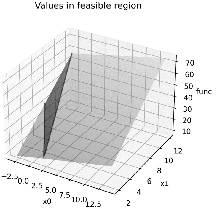
Figure 9.1 – The values of the linear function with the feasible region highlighted

As we can see, the minimum value that lies within this shaded region occurs at the intersection of the two critical lines.

8. Next, we use linprog to solve the constrained minimization problem with the bounds we created in step 1. We print the resulting object in the terminal:

   res = optimize.linprog(c, A_ub=A, b_ub=b,

       bounds= (x0_bounds, x1_bounds))

   print(res)
9. Finally, we plot the minimum function value on top of the feasible region:

   ax.plot([res.x[0]], [res.x[1]], [res.fun], "kx")

The updated plot can be seen in the following diagram:

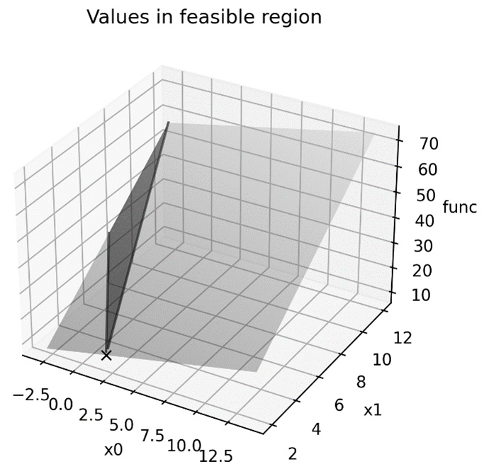
Figure 9.2 – The minimum value plotted on the feasible region

Here, we can see that the linprog routine has indeed found that the minimum is at the intersection of the two critical lines.

How it works...

Constrained linear minimization problems are common in economic situations, where you try to minimize costs while maintaining other aspects of the parameters. In fact, a lot of the terminology from optimization theory mirrors this fact. A very simple algorithm for solving these kinds of problems is called the simplex method, which uses a sequence of array operations to find the minimal solution. Geometrically, these operations represent changing to different vertices of a simplex (which we won’t define here), and it is this that gives the algorithm its name.

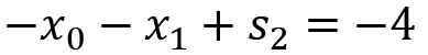
Before we continue, we’ll provide a brief outline of the process used by the simplex method to solve a constrained linear optimization problem. The problem, as presented to us, is not a matrix equation problem but a matrix inequality problem. We can remedy this problem by introducing slack variables, which turn an inequality into an equality. For example, the first constraint inequality can be rewritten as follows by introducing the slack variable, :

This satisfies the desired inequality, provided that is not negative. The second constraint inequality is greater than or equal to type inequality that we must first change so that it’s of the less than or equal to type. We do this by multiplying all terms by -1. This gives us the second row of the A matrix that we defined in the recipe. After introducing a second slack variable,, we get the second equation:

From this, we can construct a matrix whose columns contain the coefficients of the two parameter variables, and and the two slack variables, and . The rows of this matrix represent the two bounding equations and the objective function. This system of equations can now be solved, using elementary row operations on this matrix, to obtain the values of and , which minimize the objective function. Since solving matrix equations is easy and fast, this means that we can minimize linear functions quickly and efficiently.

Fortunately, we don’t need to remember how to reduce our system of inequalities into a system of linear equations, since routines such as linprog do this for us. We can simply provide the bounding inequalities as a matrix and vector pair, consisting of the coefficients of each, and a separate vector that defines the objective function. The linprog routine takes care of formulating and then solving the minimization problem.

In practice, the simplex method is not the algorithm used by the linprog routine to minimize the function. Instead, linprog uses an interior point algorithm, which is more efficient. (The method can actually be set to simplex or revised-simplex by providing the method keyword argument with the appropriate method name. In the printed resulting output, we can see that it only took five iterations to reach the solution.) The resulting object that is returned by this routine contains the parameter values at which the minimum occurs, stored in the x attribute, the value of the function at this minimum value stored in the fun attribute, and various other pieces of information about the solving process. If the method had failed, then the status attribute would have contained a numerical code that described why the method failed.

In step 2 of this recipe, we created a function that represents the objective function for this problem. This function takes a single array as input, which contains the parameter space values at which the function should be evaluated. Here, we used the tensordot routine (with axes=1) from NumPy to evaluate the dot product of the coefficient vector, , with each input, . We have to be quite careful here, since the values that we pass into the function will be a 2 × 50 × 50 array in a later step. The ordinary matrix multiplication (np.dot) would not give the 50 × 50 array output that we desire in this case.

In step 5 and step 6, we computed the points on the critical lines as those points with the following equation:

We then computed the corresponding values so that we could plot the lines that lie on the plane defined by the objective function. We also need to trim the values so that we only include those that lie in the range specified in the problem. This is done by constructing the indexing array labeled I in the code, consisting of the points that lie within the boundary values.

There’s more...

This recipe covered the constrained minimization problem and how to solve it using SciPy. However, the same method can be used to solve the constrained maximization problem. This is because maximization and minimization are dual to one another, in the sense that maximizing a function,, is the same as minimizing the function and then taking the negative of this value. In fact, we used this fact in this recipe to change the second constraining inequality from ≥ to ≤.

In this recipe, we solved a problem with only two parameter variables, but the same method will work (except for the plotting steps) for a problem involving more than two such variables. We just need to add more rows and columns to each of the arrays to account for this increased number of variables – this includes the tuple of bounds supplied to the routine. The routine can also be used with sparse matrices, where appropriate, for extra efficiency when dealing with very large amounts of variables.

The linprog routine gets its name from linear programming, which is used to describe problems of this type – finding values of that satisfy some matrix inequalities subject to other conditions. Since there is a very close connection between the theory of matrices and linear algebra, there are many very fast and efficient techniques available for linear programming problems that are not available in a non-linear context.

Minimizing a non-linear function

In the previous recipe, we saw how to minimize a very simple linear function. Unfortunately, most functions are not linear and usually don’t have nice properties that we would like. For these non-linear functions, we cannot use the fast algorithms that have been developed for linear problems, so we need to devise new methods that can be used in these more general cases. The algorithm that we will use here is called the Nelder-Mead algorithm, which is a robust and general-purpose method that’s used to find the minimum value of a function and does not rely on its gradient.

In this recipe, we’ll learn how to use the Nelder-Mead simplex method to minimize a non-linear function containing two variables.

Getting ready

In this recipe, we will use the NumPy package imported as np, the Matplotlib pyplot module imported as plt, the Axes3D class imported from mpl_toolkits.mplot3d to enable 3D plotting, and the SciPy optimize module:

import numpy as np
import matplotlib.pyplot as plt
from mpl_toolkits.mplot3d import Axes3D
from scipy import optimize

Let’s see how to use these tools to solve a non-linear optimization problem.

How to do it...

The following steps show you how to use the Nelder-Mead simplex method to find the minimum of a general non-linear objective function:

1. Define the objective function that we will minimize:

   def func(x):

       return ((x[0] - 0.5)**2 + (

           x[1] + 0.5)**2)*np.cos(0.5*x[0]*x[1])
2. Next, create a grid of values that we can plot our objective function on:

   x_r = np.linspace(-1, 1)

   y_r = np.linspace(-2, 2)

   x, y = np.meshgrid(x_r, y_r)
3. Now, we evaluate the function on this grid of points:

   z = func([x, y])
4. Next, we create a new figure with a 3d axes object and set the axis labels and the title:

   fig = plt.figure(tight_layout=True)

   ax = fig.add_subplot(projection="3d")

   ax.tick_params(axis="both", which="major", labelsize=9)

   ax.set(xlabel="x", ylabel="y", zlabel="z")

   ax.set_title("Objective function")
5. Now, we can plot the objective function as a surface on the axes we just created:

   ax.plot_surface(x, y, z, cmap="gray",

       vmax=8.0, alpha=0.5)
6. We choose an initial point that our minimization routine will start its iteration at and plot this on the surface:

   x0 = np.array([-0.5, 1.0])

   ax.plot([x0[0]], [x0[1]], func(x0), "k*")

The plot of the objective function’s surface, along with the initial point, can be seen in the following diagram. Here, we can see that the minimum value appears to occur at around 0.5 on the x axis and -0.5 on the y axis:

Figure 9.3 – A non-linear objective function with a starting point

7. Now, we use the minimize routine from the optimize package to find the minimum value and print the result object that it produces:

   result = optimize.minimize(

       func, x0, tol=1e-6, method= "Nelder-Mead")

   print(result)
8. Finally, we plot the minimum value found by the minimize routine on top of the objective function surface:

   ax.plot([result.x[0]], [result.x[1]], [result.fun], "kx")

The updated plot of the objective function, including the minimum point found by the minimize routine, can be seen in the following diagram:

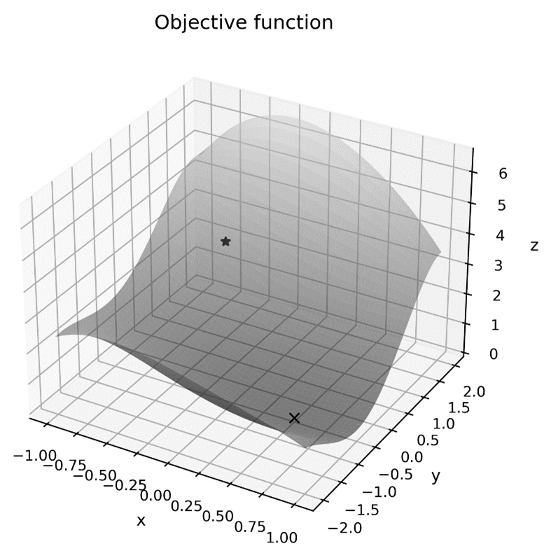
Figure 9.4 – An objective function with a starting point and a minimum point

This shows that the method has indeed found the minimum point (bottom right) within the region starting from the initial point (top left).

How it works...

The Nelder-Mead simplex method – not to be confused with the simplex method for linear optimization problems – is a simple algorithm for finding the minimum values of a non-linear function and works even when the objective function does not have a known derivative. (This is not the case for the function in this recipe; the only gain from using a gradient-based method is the speed of convergence.) The method works by comparing the values of the objective function at the vertices of a simplex, which is a triangle in a two-dimensional space. The vertex with the largest function value is reflected through the opposite edge and performs an appropriate expansion or contraction that, in effect, moves the simplex downhill.

The minimize routine from the SciPy optimize module is an entry point for many non-linear function minimization algorithms. In this recipe, we used the Nelder-Mead simplex algorithm, but there are also a number of other algorithms available. Many of these algorithms require knowledge of the gradient of the function, which might be computed automatically by the algorithm. The algorithm can be used by providing the appropriate name to the method keyword argument.

The result object that’s returned by the minimize routine contains lots of information about the solution that has been found – or not found, if an error occurred – by the solver. In particular, the desired parameters that the calculated minimum occurs at are stored in the x attribute of the result, while the value of the function is stored in the fun attribute.

The minimize routine requires the function and a starting value of x0. In this recipe, we also provided a tolerance value that the minimum should be computed at using the tol keyword argument. Changing this value will modify the accuracy of the computed solution.

There’s more...

The Nelder-Mead algorithm is an example of a gradient-free minimization algorithm, since it does not require any information about the gradient (derivative) of the objective function. There are several such algorithms, all of which typically involve evaluating the objective function at several points, and then using this information to move toward the minimum value. In general, gradient-free methods tend to converge more slowly than gradient-descent models. However, they can be used for almost any objective function, even where it is not easy to compute the gradient either exactly or by means of approximation.

Optimizing the functions of a single variable is generally easier than the multidimensional case and has its own special function in the SciPy optimize library. The minimize_scalar routine performs minimization for functions of a single variable and should be used instead of minimize in this case.

Using gradient descent methods in optimization

In the previous recipe, we used the Nelder-Mead simplex algorithm to minimize a non-linear function containing two variables. This is a fairly robust method that works even if very little is known about the objective function. However, in many situations, we do know more about the objective function, and this fact allows us to devise faster and more efficient algorithms for minimizing the function. We can do this by making use of properties such as the gradient of the function.

The gradient of a function of more than one variable describes the rate of change of the function in each of its component directions. This is a vector of the partial derivatives of the function with respect to each of the variables. From this gradient vector, we can deduce the direction in which the function is increasing most rapidly and, conversely, the direction in which the function is decreasing most rapidly from any given position. This gives us the basis for gradient descent methods for minimizing a function. The algorithm is very simple: given a starting position,, we compute the gradient at and the corresponding direction in which the gradient is most rapidly decreasing, and then make a small step in that direction. After a few iterations, this will move from the starting position to the minimum of the function.

In this recipe, we will learn how to implement an algorithm based on the steepest descent algorithm to minimize an objective function within a bounded region.

Getting ready

For this recipe, we will need the NumPy package imported as np, the Matplotlib pyplot module imported as plt, and the Axes3D object imported from mpl_toolkits.mplot3d:

import numpy as np
import matplotlib.pyplot as plt
from mpl_toolkits.mplot3d import Axes3D

Let’s implement a simple gradient descent algorithm and use it to solve the minimization problem described in the previous recipe to see how it works.

How to do it...

In the following steps, we will implement a simple gradient descent method to minimize an objective function with a known gradient function (we’re actually going to use a generator function so that we can see the method as it works):

1. We will start by defining a descend routine, which will carry out our algorithm. The function declaration is as follows:

   def descend(func,x0,grad,bounds,tol=1e-8,max_iter=100):
2. Next, we need to implement this routine. We start by defining the variables that will hold the iterate values while the method is running:

       xn = x0

       previous = np.inf

       grad_xn = grad(x0)
3. We then start our loop, which will run the iterations. We immediately check whether we are making meaningful progress before continuing:

       for i in range(max_iter):

           if np.linalg.norm(xn - previous) < tol:

               break
4. The direction is minus the gradient vector. We compute this once and store it in the direction variable:

           direction = -grad_xn
5. Now, we update the previous and current values, xnm1 and xn respectively, ready for the next iteration. This concludes the code for the descend routine:

           previous = xn

           xn = xn + 0.2*direction
6. Now, we can compute the gradient at the current value and yield all the appropriate values:

           grad_xn = grad(xn)

           yield i, xn, func(xn), grad_xn

This concludes the definition of the descend routine.

7. We can now define a sample objective function to minimize:

   def func(x):

       return ((x[0] - 0.5)**2 + (

           x[1] + 0.5)**2)*np.cos(0.5*x[0]*x[1])
8. Next, we create a grid that we will evaluate and then plot the objective function on:

   x_r = np.linspace(-1, 1)

   y_r = np.linspace(-2, 2)

   x, y = np.meshgrid(x_r, y_r)
9. Once the grid has been created, we can evaluate our function and store the result in the z variable:

   z = func([x, y])
10. Next, we create a three-dimensional surface plot of the objective function:

    surf_fig = plt.figure(tight_layout=True)

    surf_ax = surf_fig.add_subplot(projection="3d")

    surf_ax.tick_params(axis="both", which="major",

        labelsize=9)

    surf_ax.set(xlabel="x", ylabel="y", zlabel="z")

    surf_ax.set_title("Objective function")

    surf_ax.plot_surface(x, y, z, cmap="gray", 

        vmax=8.0, alpha=0.5)
11. Before we can start the minimization process, we need to define an initial point, x0. We plot this point on the objective function plot we created in the previous step:

    x0 = np.array([-0.8, 1.3])

    surf_ax.plot([x0[0]], [x0[1]], func(x0), "k*")

The surface plot of the objective function, along with the initial value, can be seen in the following diagram:

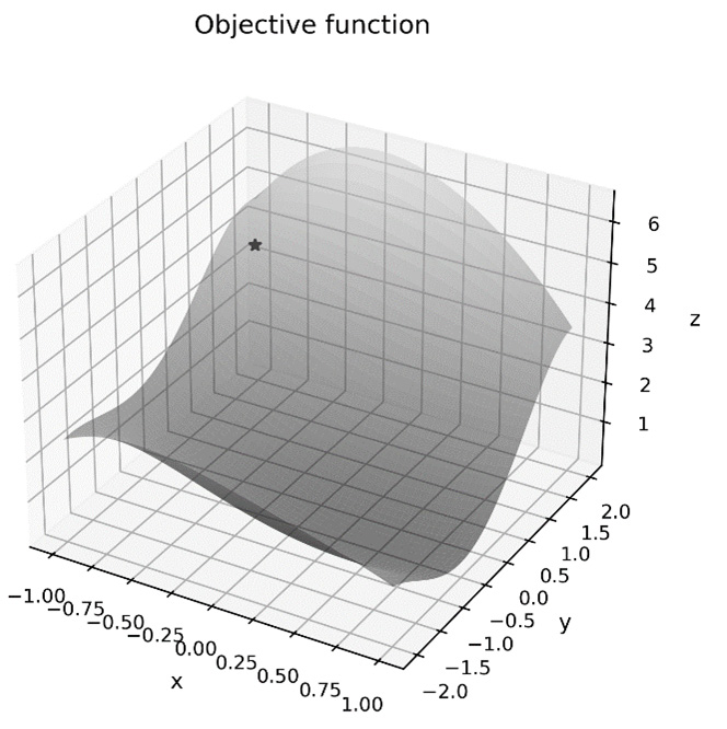
Figure 9.5 – The surface of the objective function with the initial position

12. Our descend routine requires a function that evaluates the gradient of the objective function, so we will define one:

    def grad(x):

        c1 = x[0]**2 - x[0] + x[1]**2 + x[1] + 0.5

        cos_t = np.cos(0.5*x[0]*x[1])

        sin_t = np.sin(0.5*x[0]*x[1])

        return np.array([

            (2*x[0]-1)*cos_t - 0.5*x[1]*c1*sin_t,

            (2*x[1]+1)*cos_t - 0.5*x[0]*c1*sin_t

        ])
13. We will plot the iterations on a contour plot, so we set this up as follows:

    cont_fig, cont_ax = plt.subplots()

    cont_ax.set(xlabel="x", ylabel="y")

    cont_ax.set_title("Contour plot with iterates")

    cont_ax.contour(x, y, z, levels=25, cmap="gray",

        vmax=8.0, opacity=0.6)
14. Now, we create a variable that holds the bounds in the and directions as a tuple of tuples. These are the same bounds from the linspace calls in step 10:

    bounds = ((-1, 1), (-2, 2))
15. We can now use a for loop to drive the descend generator to produce each of the iterations and add the steps to the contour plot:

    xnm1 = x0

    for i, xn, fxn, grad_xn in descend(func, x0, grad, bounds):

        cont_ax.plot([xnm1[0], xn[0]], [xnm1[1], xn[1]],           	        "k*--")

        xnm1, grad_xnm1 = xn, grad_xn
16. Once the loop is complete, we print the final values to the Terminal:

    print(f"iterations={i}")

    print(f"min val at {xn}")

    print(f"min func value = {fxn}")

The output of the preceding print statements is as follows:

iterations=37
min val at [ 0.49999999 -0.49999999]
min func value = 2.1287163880894953e-16

Here, we can see that our routine used 37 iterations to find a minimum at approximately (0.5, -0.5), which is correct.

The contour plot with its iterations plotted can be seen in the following diagram:

Figure 9.6 – A contour plot of the objective function with the gradient descent iterating to a minimum value

Here, we can see that the direction of each iteration – shown by the dashed lines – is in the direction where the objective function is decreasing most rapidly. The final iteration lies at the center of the bowl of the objective function, which is where the minimum occurs.

How it works...

The heart of this recipe is the descend routine. The process that’s defined in this routine is a very simple implementation of the gradient descent method. Computing the gradient at a given point is handled by the grad argument, which is then used to deduce the direction of travel for the iteration by taking direction = -grad. We multiply this direction by a fixed scale factor (sometimes called the learning rate) with a value of 0.2 to obtain the scaled step, and then take this step by adding 0.2*direction to the current position.

The solution in the recipe took 37 iterations to converge, which is a mild improvement on the Nelder-Mead simplex algorithm from the Minimizing a non-linear function recipe, which took 58 iterations. (This is not a perfect comparison, since we changed the starting position for this recipe.) This performance is heavily dependent on the step size that we choose. In this case, we fixed the maximum step size to be 0.2 times the size of the direction vector. This keeps the algorithm simple, but it is not particularly efficient.

In this recipe, we chose to implement the algorithm as a generator function so that we could see the output of each step and plot this on our contour plot as we stepped through the iteration. In practice, we probably wouldn’t want to do this and instead return the calculated minimum once the iterations have finished. To do this, we can simply remove the yield statement and replace it with return xn at the very end of the function, at the main function’s indentation (that is, not inside the loop). If you want to guard against non-convergence, you can use the else feature of the for loop to catch cases where the loop finishes because it has reached the end of its iterator without hitting the break keyword. This else block could raise an exception to indicate that the algorithm has failed to stabilize to a solution. The condition we used to end the iteration in this recipe does not guarantee that the method has reached a minimum, but this will usually be the case.

There’s more...

In practice, you would not usually implement the gradient descent algorithm for yourself and instead use a general-purpose routine from a library such as the SciPy optimize module. We can use the same minimize routine that we used in the previous recipe to perform minimization with a variety of different algorithms, including several gradient descent algorithms. These implementations are likely to have much higher performance and be more robust than a custom implementation such as this.

The gradient descent method we used in this recipe is a very naive implementation and can be greatly improved by allowing the routine to choose the step size at each step. (Methods that are allowed to choose their own step size are sometimes called adaptive methods.) The difficult part of this improvement is choosing the size of the step to take in this direction. For this, we need to consider the function of a single variable, which is given by the following equation:

Here, represents the current point, represents the current direction, and is a parameter. For simplicity, we can use a minimization routine called minimize_scalar for scalar-valued functions from the SciPy optimize module. Unfortunately, it is not quite as simple as passing in this auxiliary function and finding the minimum value. We have to bound the possible value of so that the computed minimizing point, , lies within the region that we are interested in.

To understand how we bound the values of , we must first look at the construction geometrically. The auxiliary function that we introduce evaluates the objective function along a single line in the given direction. We can picture this as taking a single cross section through the surface that passes through the current point in the direction. The next step of the algorithm is finding the step size, , that minimizes the values of the objective function along this line – this is a scalar function, which is much easier to minimize. The bounds should then be the range of values, during which this line lies within the rectangle defined by the and boundary values. We determine the four values at which this line crosses those and boundary lines, two of which will be negative and two of which will be positive. (This is because the current point must lie within the rectangle.) We take the minimum of the two positive values and the maximum of the two negative values and pass these bounds to the scalar minimization routine. This is achieved using the following code:

alphas = np.array([
    (bounds[0][0] - xn[0]) / direction[0],
    # x lower
   (bounds[1][0] - xn[1]) / direction[1],
    # y lower
    (bounds[0][1] - xn[0]) / direction[0],
    # x upper
    (bounds[1][1] - xn[1]) / direction[1] 
    # y upper
])
alpha_max = alphas[alphas >= 0].min()
alpha_min = alphas[alphas < 0].max()
result = minimize_scalar(lambda t: 
    func(xn + t*direction),
    method="bounded",
    bounds=(alpha_min, alpha_max))
amount = result.x

Once the step size has been chosen, the only remaining step is to update the current xn value, as follows:

xn = xn + amount * direction

Using this adaptive step size increases the complexity of the routine, but the performance is massively improved. Using this revised routine, the method converged in just three iterations, which is far fewer than the number of iterations used by the naive code in this recipe (37 iterations) or by the Nelder-Mead simplex algorithm in the previous recipe (58 iterations). This reduction in the number of iterations is exactly what we expected by providing the method with more information in the form of the gradient function.

We created a function that returned the gradient of the function at a given point. We computed this gradient by hand before we started, which will not always be easy or even possible. Instead, it is much more common to replace the analytic gradient used here with a numerically computed gradient that’s been estimated using finite differences or a similar algorithm. This has an impact on performance and accuracy, as all approximations do, but these concerns are usually minor given the improvement in the speed of convergence offered by gradient descent methods.

Gradient descent-type algorithms are particularly popular in machine learning applications. Most of the popular Python machine learning libraries – including PyTorch, TensorFlow, and Theano – offer utilities for automatically computing gradients numerically for data arrays. This allows gradient descent methods to be used in the background to improve performance.

A popular variation of the gradient descent method is stochastic gradient descent, where the gradient is estimated by sampling randomly rather than using the whole set of data. This can dramatically reduce the computational burden of the method – at the cost of slower convergence – especially for high-dimensional problems such as those that are common in machine learning applications. Stochastic gradient descent methods are often combined with backpropagation to form the basis for training artificial neural networks in machine learning applications.

There are several extensions of the basic stochastic gradient descent algorithm. For example, the momentum algorithm incorporates the previous increment into the calculation of the next increment. Another example is the adaptive gradient algorithm, which incorporates per-parameter learning rates to improve the rate of convergence for problems that involve a large number of sparse parameters.

Using least squares to fit a curve to data

Least squares is a powerful technique for finding a function from a relatively small family of potential functions that best describe a particular set of data. This technique is especially common in statistics. For example, least squares is used in linear regression problems – here, the family of potential functions is the collection of all linear functions. Usually, the family of functions that we try to fit has relatively few parameters that can be adjusted to solve the problem.

The idea of least squares is relatively simple. For each data point, we compute the square of the residual – the difference between the value of the point and the expected value given a function – and try to make the sum of these squared residuals as small as possible (hence, least squares).

In this recipe, we’ll learn how to use least squares to fit a curve to a sample set of data.

Getting ready

For this recipe, we will need the NumPy package imported, as usual, as np, and the Matplotlib pyplot module imported as plt:

import numpy as np
import matplotlib.pyplot as plt

We will also need an instance of the default random number generator from the NumPy random module imported, as follows:

from numpy.random import default_rng
rng = default_rng(12345)

Finally, we need the curve_fit routine from the SciPy optimize module:

from scipy.optimize import curve_fit

Let’s see how to use this routine to fit a non-linear curve to some data.

How to do it...

The following steps show you how to use the curve_fit routine to fit a curve to a set of data:

1. The first step is to create the sample data:

   SIZE = 100

   x_data = rng.uniform(-3.0, 3.0, size=SIZE)

   noise = rng.normal(0.0, 0.8, size=SIZE)

   y_data = 2.0*x_data**2 - 4*x_data + noise
2. Next, we produce a scatter plot of the data to see whether we can identify the underlying trend in the data:

   fig, ax = plt.subplots()

   ax.scatter(x_data, y_data)

   ax.set(xlabel="x", ylabel="y",

       title="Scatter plot of sample data")

The scatter plot that we have produced can be seen in the following diagram. Here, we can see that the data certainly doesn’t follow a linear trend (straight line). Since we know the trend is a polynomial, our next guess would be a quadratic trend. This is what we’re using here:

Figure 9.7 – Scatter plot of the sample data – we can see that it does not follow a linear trend

3. Next, we create a function that represents the model that we wish to fit:

   def func(x, a, b, c):

       return a*x**2 + b*x + c
4. Now, we can use the curve_fit routine to fit the model function to the sample data:

   coeffs, _ = curve_fit(func, x_data, y_data)

   print(coeffs)

   # [ 1.99611157 -3.97522213 0.04546998]
5. Finally, we plot the best fit curve on top of the scatter plot to evaluate how well the fitted curve describes the data:

   x = np.linspace(-3.0, 3.0, SIZE)

   y = func(x, coeffs[0], coeffs[1], coeffs[2])

   ax.plot(x, y, "k--")

The updated scatter plot can be seen in the following diagram:

Figure 9.8 – A scatter plot with the curve of the best fit found using superimposed least squares

Here, we can see that the curve we have found fits the data reasonably well. The coefficients are not exactly equal to the true model – this is the effect of the added noise.

How it works...

The curve_fit routine performs least-squares fitting to fit the model’s curve to the sample data. In practice, this amounts to minimizing the following objective function:

Here, the pairs are the points from the sample data. In this case, we are optimizing over a three-dimensional parameter space, with one dimension for each of the parameters. The routine returns the estimated coefficients – the point in the parameter space at which the objective function is minimized – and a second variable that contains estimates for the covariance matrix for the fit. We ignored this in this recipe.

The estimated covariance matrix that’s returned from the curve_fit routine can be used to give a confidence interval for the estimated parameters. This is done by taking the square root of the diagonal elements divided by the sample size (100 in this recipe). This gives the standard error for the estimate that, when multiplied by the appropriate values corresponding to the confidence, gives us the size of the confidence interval. (We discussed confidence intervals in Chapter 6, Working with Data and Statistics.)

You might have noticed that the parameters estimated by the curve_fit routine are close, but not exactly equal, to the parameters that we used to define the sample data in step 1. The fact that these are not exactly equal is due to the normally distributed noise that we added to the data. In this recipe, we knew that the underlying structure of the data was quadratic – that is, a degree 2 polynomial – and not some other, more esoteric, function. In practice, we are unlikely to know so much about the underlying structure of the data, which is the reason we added noise to the sample.

There’s more...

There is another routine in the SciPy optimize module for performing least-squares fitting called least_squares. This routine has a slightly less intuitive signature but does return an object containing more information about the optimization process. However, the way this routine is set up is perhaps more similar to the way that we constructed the underlying mathematical problem in the How it works... section. To use this routine, we define the objective function as follows:

def func(params, x, y):
    return y -(
        params[0]*x**2 + params[1]*x + params[2])

We pass this function along with a starting estimate in the parameter space, x0, such as (1, 0, 0). The additional parameters for the objective function, func, can be passed using the args keyword argument – for example, we could use args=(x_data, y_data). These arguments are passed into the x and y arguments of the objective function. To summarize, we could have estimated the parameters using the following call to least_squares:

results = least_squares(func, [1, 0, 0], args=(x_data, y_data))

The results object that’s returned from the least_squares routine is actually the same as the one returned by the other optimization routines described in this chapter. It contains details such as the number of iterations used, whether the process was successful, detailed error messages, the parameter values, and the value of the objective function at the minimum value.

Analyzing simple two-player games

Game theory is a branch of mathematics concerned with the analysis of decision-making and strategy. It has applications in economics, biology, and behavioral science. Many seemingly complex situations can be reduced to a relatively simple mathematical game that can be analyzed in a systematic way to find optimal solutions.

A classic problem in game theory is the prisoner’s dilemma, which, in its original form, is as follows: two co-conspirators are caught and must decide whether to remain quiet or to testify against the other. If both remain quiet, they both serve a 1-year sentence; if one testifies but the other does not, the testifier is released and the other serves a 3-year sentence; and if both testify against one another, they both serve a 2-year sentence. What should each conspirator do? It turns out that the best choice each conspirator can make, given any reasonable distrust of the other, is to testify. Adopting this strategy, they will either serve no sentence or a 2-year sentence maximum.

Since this book is about Python, we will use a variation of this classic problem to illustrate just how universal the idea of this problem is. Consider the following problem: you and your colleague have to write some code for a client. You think that you could write the code faster in Python, but your colleague thinks that they could write it faster in C. The question is, which language should you choose for the project?

You think that you could write the Python code four times faster than in C, so you write C with speed 1 and Python with speed 4. Your colleague says that they can write C slightly faster than Python, so they write C with speed 3 and Python with speed 2. If you both agree on a language, then you write the code at the speed you predicted, but if you disagree, then the productivity of the faster programmer is reduced by 1. We can summarize this as follows:

Figure 9.9 – A table of the predicted work speed in various configurations

In this recipe, we will learn how to construct an object in Python to represent this simple two-player game, and then perform some elementary analysis regarding the outcomes of this game.

Getting ready

For this recipe, we will need the NumPy package imported as np, and the Nashpy package imported as nash:

import numpy as np
import nashpy as nash

Let’s see how to use the nashpy package to analyze a simple two-player game.

How to do it...

The following steps show you how to create and perform some simple analysis of a two-player game using Nashpy:

1. First, we need to create matrices that hold the payoff information for each player (you and your colleague, in this example):

   you = np.array([[1, 3], [1, 4]])

   colleague = np.array([[3, 2], [2, 2]])
2. Next, we create a Game object that holds the game represented by these payoff matrices:

   dilemma = nash.Game(you, colleague)
3. We compute the utility for the given choices using index notation:

   print(dilemma[[1, 0], [1, 0]])      # [1 3]

   print(dilemma[[1, 0], [0, 1]])      # [3 2]

   print(dilemma[[0, 1], [1, 0]])      # [1 2]

   print(dilemma[[0, 1], [0, 1]])      # [4 2]
4. We can also compute the expected utilities based on the probabilities of making a specific choice:

   print(dilemma[[0.1, 0.9], [0.5, 0.5]]) # [2.45 2.05]

These expected utilities represent what we’d expect (on average) to see if we repeated the game numerous times with the specified probabilities.

How it works...

In this recipe, we built a Python object that represents a very simple two-player strategic game. The idea here is that there are two players who have decisions to make, and each combination of both players’ choices gives a specific payoff value. What we’re aiming to do here is find the best choice that each player can make. The players are assumed to make a single move simultaneously, in the sense that neither is aware of the other’s choice. Each player has a strategy that determines the choice they make.

In step 1, we create two matrices – one for each player – that are assigned to each combination of choices for the payoff value. These two matrices are wrapped by the Game class from Nashpy, which provides a convenient and intuitive (from a game-theoretic point of view) interface for working with games. We can quickly calculate the utility of a given combination of choices by passing in the choices using index notation.

We can also calculate expected utilities based on a strategy where choices are chosen at random according to some probability distribution. The syntax is the same as for the deterministic case described previously, except we provide a vector of probabilities for each choice. We compute the expected utilities based on the probability that you choose Python 90% of the time, while your colleague chooses Python 50% of the time. The expected speeds are 2.45 and 2.05 for you and your colleague respectively.

There’s more...

There is an alternative to computational game theory in Python. The Gambit project is a collection of tools used for computation in game theory that has a Python interface (http://www.gambit-project.org/). This is a mature project built around C libraries and offers more performance than Nashpy.

Computing Nash equilibria

A Nash equilibrium is a two-player strategic game – similar to the one we saw in the Analyzing simple two-player games recipe – that represents a steady state in which every player sees the best possible outcome. However, this doesn’t mean that the outcome linked to a Nash equilibrium is the best overall. Nash equilibria are more subtle than this. An informal definition of a Nash equilibrium is as follows: an action profile in which no individual player can improve their outcome, assuming that all other players adhere to the profile.

We will explore the notion of a Nash equilibrium with the classic game of rock-paper-scissors. The rules are as follows. Each player can choose one of the options: rock, paper, or scissors. Rock beats scissors, but loses to paper; paper beats rock, but loses to scissors; scissors beats paper, but loses to rock. Any game in which both players make the same choice is a draw. Numerically, we represent a win by +1, a loss by -1, and a draw by 0. From this, we can construct a two-player game and compute Nash equilibria for this game.

In this recipe, we will compute Nash equilibria for the classic game of rock-paper-scissors.

Getting ready

For this recipe, we will need the NumPy package imported as np, and the Nashpy package imported as nash:

import numpy as np
import nashpy as nash

Let’s see how to use the nashpy package to compute Nash equilibria for a two-player strategy game.

How to do it...

The following steps show you how to compute Nash equilibria for a simple two-player game:

1. First, we need to create a payoff matrix for each player. We will start with the first player:

   rps_p1 = np.array([

       [ 0, -1, 1], # rock payoff

       [ 1, 0, -1], # paper payoff

       [-1, 1, 0] # scissors payoff

   ])
2. The payoff matrix for the second player is the transpose of rps_p1:

   rps_p2 = rps_p1.transpose()
3. Next, we create the Game object to represent the game:

   rock_paper_scissors = nash.Game(rps_p1, rps_p2)
4. We compute the Nash equilibria for the game using the support enumeration algorithm:

   equilibria = rock_paper_scissors.support_enumeration()
5. We iterate over the equilibria and print the profile for each player:

   for p1, p2 in equilibria:

       print("Player 1", p1)

       print("Player 2", p2)

The output of these print statements is as follows:

Player 1 [0.33333333 0.33333333 0.33333333]
Player 2 [0.33333333 0.33333333 0.33333333]

How it works...

Nash equilibria are extremely important in game theory because they allow us to analyze the outcomes of strategic games and identify advantageous positions. They were first described by John F. Nash in 1950 and have played a pivotal role in modern game theory. A two-player game may have many Nash equilibria, but any finite two-player game must have at least one. The problem is finding all the possible Nash equilibria for a given game.

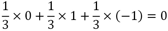
In this recipe, we used the support enumeration, which effectively enumerates all possible strategies and filters down to those that are Nash equilibria. In this recipe, the support enumeration algorithm found just one Nash equilibrium, which is a mixed strategy. This means that the only strategy for which there is no improvement involves picking one of the choices at random, each with a 1/3 probability. This is hardly a surprise to anyone who has played rock-paper-scissors, since for any choice we make, our opponent has a 1 in 3 chance of choosing (at random) the move that beats our choice. Equally, we have a 1 in 3 chance of drawing or winning the game, so our expected value over all these possibilities is as follows:

Without knowing exactly which of the choices our opponent will choose, there is no way to improve this expected outcome.

There’s more...

The Nashpy package also provides other algorithms for computing Nash equilibria. Specifically, the vertex_enumeration method, when used on a Game object, uses the vertex enumeration algorithm, while the lemke_howson_enumeration method uses the Lemke-Howson algorithm. These alternative algorithms have different characteristics and may be more efficient for some problems.

See also

The documentation for the Nashpy package contains more detailed information about the algorithms and game theory involved. This includes a number of references to texts on game theory. This documentation can be found at https://nashpy.readthedocs.io/en/latest/.

Further reading

As usual, the Numerical Recipes book is a good source of numerical algorithms. Chapter 10, Minimization or Maximization of Functions, deals with the maximization and minimization of functions:

• Press, W.H., Teukolsky, S.A., Vetterling, W.T., and Flannery, B.P., 2017. Numerical recipes: the art of scientific computing. 3rd ed. Cambridge: Cambridge University Press.

More specific information on optimization can be found in the following books:

• Boyd, S.P. and Vandenberghe, L., 2018. Convex optimization. Cambridge: Cambridge University Press.
• Griva, I., Nash, S., and Sofer, A., 2009. Linear and nonlinear optimization. 2nd ed. Philadelphia: Society for Industrial and Applied Mathematics.

Finally, the following book is a good introduction to game theory:

• Osborne, M.J., 2017. An introduction to game theory. Oxford: Oxford University Press.