1

An Introduction to Basic Packages, Functions, and Concepts

Before getting started on any practical recipes, we’ll use this opening chapter to introduce several core mathematical concepts and structures and their Python representations. We’ll look at basic numerical types, basic mathematical functions (trigonometric functions, exponential function, and logarithms), and matrices. Matrices are fundamental in most computational applications because of the connection between matrices and solutions of systems of linear equations. We’ll explore some of these applications in this chapter, but matrices will play an important role throughout this book.

We’ll cover the following main topics in this order:

• Exploring Python numerical types
• Understanding basic mathematical functions
• Diving into the world of NumPy
• Working with matrices and linear algebra

NumPy arrays and the basic mathematical functions we will see in this chapter will be used throughout the rest of the book—they appear in essentially every recipe. Matrix theory, and other topics discussed here, underpin many of the computational methods that are used behind the scenes in packages discussed in this book. Some other topics are important to know about, though we will not necessarily use these in recipes in the book (for example, the alternative numerical types).

Technical requirements

In this chapter, and throughout this book, we will use Python version 3.10, which is the most recent version of Python at the time of writing. Most of the code in this book will work on recent versions of Python from 3.6. We will use features that were introduced in Python 3.6 at various points, including f-strings. This means that you may need to change python3.10, which appears in any terminal commands, to match your version of Python. This might be another version of Python, such as python3.6 or python3.7, or a more general command such as python3 or python. For the latter commands, you need to check that the version of Python is at least 3.6 by using the following command:

python --version

Python has built-in numerical types and basic mathematical functions that suffice for small applications that involve only small calculations. The NumPy package provides a high-performance array type and associated routines (including basic mathematical functions that operate efficiently on arrays). This package will be used in many of the recipes in this chapter and the remainder of this book. We will also make use of the SciPy package in the latter recipes of this chapter. Both can be installed using your preferred package manager, such as pip:

python3.10 -m pip install numpy scipy

By convention, we import these packages under a shorter alias. We import numpy as np and scipy as sp using the following import statements:

import numpy as np
import scipy as sp

These conventions are used in the official documentation (https://numpy.org/doc/stable/ and https://docs.scipy.org/doc/scipy/) for these packages, along with many tutorials and other materials that use these packages.

The code for this chapter can be found in the Chapter 01 folder of the GitHub repository at https://github.com/PacktPublishing/Applying-Math-with-Python-2nd-Edition/tree/main/Chapter%2001.

Exploring Python numerical types

Python provides basic numerical types such as arbitrarily sized integers and floating-point numbers (double precision) as standard, but it also provides several additional types that are useful in specific applications where precision is especially important. Python also provides (built-in) support for complex numbers, which is useful for some more advanced mathematical applications. Let’s take a look at some of these different numerical types, starting with the Decimal type.

Decimal type

For applications that require decimal digits with accurate arithmetic operations, use the Decimal type from the decimal module in the Python Standard Library:

from decimal import Decimal
num1 = Decimal('1.1')
num2 = Decimal('1.563')
num1 + num2  # Decimal('2.663')

Performing this calculation with float objects gives the result 2.6630000000000003, which includes a small error arising from the fact that certain numbers cannot be represented exactly using a finite sum of powers of 2. For example, 0.1 has a binary expansion 0.000110011..., which does not terminate. Any floating-point representation of this number will therefore carry a small error. Note that the argument to Decimal is given as a string rather than a float.

The Decimal type is based on the IBM General Decimal Arithmetic Specification (http://speleotrove.com/decimal/decarith.html), which is an alternative specification for floating-point arithmetic that represents decimal numbers exactly by using powers of 10 rather than powers of 2. This means that it can be safely used for calculations in finance where the accumulation of rounding errors would have dire consequences. However, the Decimal format is less memory efficient, since it must store decimal digits rather than binary digits (bits), and these are more computationally expensive than traditional floating-point numbers.

The decimal package also provides a Context object, which allows fine-grained control over the precision, display, and attributes of Decimal objects. The current (default) context can be accessed using the getcontext function from the decimal module. The Context object returned by getcontext has a number of attributes that can be modified. For example, we can set the precision for arithmetic operations:

from decimal import getcontext
ctx = getcontext()
num = Decimal('1.1')
num**4  # Decimal('1.4641')
ctx.prec = 4 # set new precision
num**4  # Decimal('1.464')

When we set the precision to 4, rather than the default 28, we see that the fourth power of 1.1 is rounded to four significant figures.

The context can even be set locally by using the localcontext function, which returns a context manager that restores the original environment at the end of the with block:

from decimal import localcontext
num = Decimal("1.1")
with localcontext() as ctx:
    ctx.prec = 2
    num**4  # Decimal('1.5')
num**4  # Decimal('1.4641')

This means that the context can be freely modified inside the with block, and will be returned to the default at the end.

Fraction type

Alternatively, for working with applications that require accurate representations of integer fractions, such as when working with proportions or probabilities, there is the Fraction type from the fractions module in the Python Standard Library. The usage is similar, except that we typically give the numerator and denominator of the fraction as arguments:

from fractions import Fraction
num1 = Fraction(1, 3)
num2 = Fraction(1, 7)
num1 * num2  # Fraction(1, 21)

The Fraction type simply stores two integers—the numerator and the denominator—and arithmetic is performed using the basic rules for the addition and multiplication of fractions.

Complex type

The square root function works fine for positive numbers but isn’t defined for negative numbers. However, we can extend the set of real numbers by formally adding a symbol, i—the imaginary unit—whose square is (that is, ). A complex number is a number of the form , where and are real numbers (those that we are used to). In this form, the number is called the real part, and is called the imaginary part. Complex numbers have their own arithmetic (addition, subtraction, multiplication, division) that agrees with the arithmetic of real numbers when the imaginary part is zero. For example, we can add the complex numbers and to get , or multiply them together to get the following:

Complex numbers appear more often than you might think, and are often found behind the scenes when there is some kind of cyclic or oscillatory behavior. This is because the and trigonometric functions are the real and imaginary parts, respectively, of the complex exponential:

Here, is any real number. The details, and many more interesting facts and theories of complex numbers, can be found in many resources covering complex numbers. The following Wikipedia page is a good place to start: https://en.wikipedia.org/wiki/Complex_number.

Python has support for complex numbers, including a literal character to denote the complex unit 1j in code. This might be different from the idiom for representing the complex unit that you are familiar with from other sources on complex numbers. Most mathematical texts will often use the symbol to represent the complex unit:

z = 1 + 1j
z + 2  # 3 + 1j
z.conjugate()  # 1 - 1j

The complex conjugate of a complex number is the result of making the imaginary part negative. This has the effect of swapping between two possible solutions to the equation .

Special complex number-aware mathematical functions are provided in the cmath module of the Python Standard Library.

Now that we have seen some of the basic mathematical types that Python has to offer, we can start to explore some of the mathematical functions that it provides.

Understanding basic mathematical functions

Basic mathematical functions appear in many applications. For example, logarithms can be used to scale data that grows exponentially to give linear data. The exponential function and trigonometric functions are common fixtures when working with geometric information, the gamma function appears in combinatorics, and the Gaussian error function is important in statistics.

The math module in the Python Standard Library provides all of the standard mathematical functions, along with common constants and some utility functions, and it can be imported using the following command:

import math

Once it’s imported, we can use any of the mathematical functions that are contained in this module. For instance, to find the square root of a non-negative number, we would use the sqrt function from math:

import math
math.sqrt(4)  #  2.0

Attempting to use the sqrt function with a negative argument will raise a value error. The square root of a negative number is not defined for this sqrt function, which deals only with real numbers. The square root of a negative number—this will be a complex number—can be found using the alternative sqrt function from the cmath module in the Python Standard Library.

The sine, cosine, and tangent trigonometric functions are available under their common abbreviations sin, cos, and tan, respectively, in the math module. The pi constant holds the value of π, which is approximately 3.1416:

theta = math.pi/4
math.cos(theta)  # 0.7071067811865476
math.sin(theta)  # 0.7071067811865475
math.tan(theta)  # 0.9999999999999999

The inverse trigonometric functions are named acos, asin, and atan in the math module:

math.asin(-1)  # -1.5707963267948966
math.acos(-1)  # 3.141592653589793
math.atan(1)  # 0.7853981633974483

The log function in the math module performs logarithms. It has an optional argument to specify the base of the logarithm (note that the second argument is positional only). By default, without the optional argument, it is the natural logarithm with base . The constant can be accessed using math.e:

math.log(10) # 2.302585092994046
math.log(10, 10) # 1.0

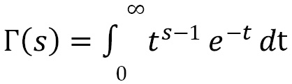
The math module also contains the gamma function, which is the gamma function, and the erf function, the Gaussian error function, which is important in statistics. Both functions are defined by integrals. The gamma function is defined by this integral:

The Gaussian error function is defined by this integral:

The integral in the definition of the error function cannot be evaluated using calculus, and instead must be computed numerically:

math.gamma(5) # 24.0
math.erf(2) # 0.9953222650189527

In addition to standard functions such as trigonometric functions, logarithms, and exponential functions, the math module contains various theoretic and combinatorial functions. These include the comb and factorial functions, which are useful in a variety of applications. The comb function called with arguments and returns the number of ways to choose items from a collection of without repeats if the order is not important. For example, picking 1 then 2 is the same as picking 2 then 1. This number is sometimes written . The factorial called with argument returns the factorial :

math.comb(5, 2)  # 10
math.factorial(5)  # 120

Applying the factorial to a negative number raises a ValueError. The factorial of an integer, , coincides with the value of the gamma function at ; that is:

The math module also contains a function that returns the greatest common divisor of its arguments called gcd. The greatest common divisor of and is the largest integer such that divides both and exactly:

math.gcd(2, 4)  # 2
math.gcd(2, 3)  # 1

There are also a number of functions for working with floating-point numbers. The fsum function performs addition on an iterable of numbers and keeps track of the sums at each step to reduce the error in the result. This is nicely illustrated by the following example:

nums = [0.1]*10  # list containing 0.1 ten times
sum(nums)  # 0.9999999999999999
math.fsum(nums)  # 1.0

The isclose function returns True if the difference between the arguments is smaller than the tolerance. This is especially useful in unit tests, where there may be small variations in results based on machine architecture or data variability.

Finally, the floor and ceil functions from math provide the floor and ceiling of their argument. The floor of a number is the largest integer with , and the ceiling of is the smallest integer with . These functions are useful when converting between a float obtained by dividing one number by another and an integer.

The math module contains functions that are implemented in C (assuming you are running CPython), and so are much faster than those implemented in Python. This module is a good choice if you need to apply a function to a relatively small collection of numbers. If you want to apply these functions to a large collection of data simultaneously, it is better to use their equivalents from the NumPy package, which is more efficient for working with arrays. In general, if you have imported the NumPy package already, then it is probably best to always use NumPy equivalents of these functions to limit the chance of error. With this in mind, let’s now introduce the NumPy package and its basic objects: multi-dimensional arrays.

Diving into the world of NumPy

NumPy provides high-performance array types and routines for manipulating these arrays in Python. These arrays are useful for processing large datasets where performance is crucial. NumPy forms the base for the numerical and scientific computing stack in Python. Under the hood, NumPy makes use of low-level libraries for working with vectors and matrices, such as the Basic Linear Algebra Subprograms (BLAS) package, to accelerate computations.

Traditionally, the NumPy package is imported under the shorter alias np, which can be accomplished using the following import statement:

import numpy as np

This convention is used in the NumPy documentation and in the wider scientific Python ecosystem (SciPy, pandas, and so on).

The basic type provided by the NumPy library is the ndarray type (henceforth referred to as a NumPy array). Generally, you won’t create your own instances of this type, and will instead use one of the helper routines such as array to set up the type correctly. The array routine creates NumPy arrays from an array-like object, which is typically a list of numbers or a list of lists (of numbers). For example, we can create a simple array by providing a list with the required elements:

arr = np.array([1, 2, 3, 4])  # array([1, 2, 3, 4])

The NumPy array type (ndarray) is a Python wrapper around an underlying C array structure. The array operations are implemented in C and optimized for performance. NumPy arrays must consist of homogeneous data (all elements have the same type), although this type could be a pointer to an arbitrary Python object. NumPy will infer an appropriate data type during creation if one is not explicitly provided using the dtype keyword argument:

np.array([1, 2, 3, 4], dtype=np.float32)
# array([1., 2., 3., 4.], dtype=float32)

NumPy offers type specifiers for numerous C-types that can be passed into the dtype parameter, such as np.float32 used previously. Generally speaking, these type specifiers are of form namexx where the name is the name of a type—such as int, float, or complex—and xx is a number of bits—for example, 8, 16, 32, 64, 128. Usually, NumPy does a pretty good job of selecting a good type for the input given, but occasionally, you will want to override it. The preceding case is a good example— without the dtype=np.float32 argument, NumPy would assume the type to be int64.

Under the hood, a NumPy array of any shape is a buffer containing the raw data as a flat (one-dimensional) array and a collection of additional metadata that specifies details such as the type of the elements.

After creation, the data type can be accessed using the dtype attribute of the array. Modifying the dtype attribute will have undesirable consequences since the raw bytes that constitute the data in the array will simply be reinterpreted as the new data type. For example, if we create an array using Python integers, NumPy will convert those to 64-bit integers in the array. Changing the dtype value will cause NumPy to reinterpret these 64-bit integers to the new data type:

arr = np.array([1, 2, 3, 4])
print(arr.dtype) # int64
arr.dtype = np.float32
print(arr)
# [1.e-45 0.e+00 3.e-45 0.e+00 4.e-45 0.e+00 6.e-45 0.e+00]

Each 64-bit integer has been re-interpreted as two 32-bit floating-point numbers, which clearly give nonsense values. Instead, if you wish to change the data type after creation, use the astype method to specify the new type. The correct way to change the data type is shown here:

arr = arr.astype(np.float32)
print(arr)
# [1. 2. 3. 4.]

NumPy also provides a number of routines for creating various standard arrays. The zeros routine creates an array of the specified shape, in which every element is 0, and the ones routine creates an array in which every element is 1.

Element access

NumPy arrays support the getitem protocol, so elements in an array can be accessed as if they were a list and support all of the arithmetic operations, which are performed component-wise. This means we can use the index notation and the index to retrieve the element from the specified index, as follows:

arr = np.array([1, 2, 3, 4])
arr[0]  # 1
arr[2]  # 3

This also includes the usual slice syntax for extracting an array of data from an existing array. A slice of an array is again an array, containing the elements specified by the slice. For example, we can retrieve an array containing the first two elements of ary, or an array containing the elements at even indexes, as follows:

first_two = arr[:2]  # array([1, 2])
even_idx = arr[::2]  # array([1, 3])

The syntax for a slice is start:stop:step. We can omit either, or both, of start and stop to take from the beginning or the end, respectively, of all elements. We can also omit the step parameter, in which case we also drop the trailing :. The step parameter describes the elements from the chosen range that should be selected. A value of 1 selects every element or, as in the recipe, a value of 2 selects every second element (starting from 0 gives even-numbered elements). This syntax is the same as for slicing Python lists.

Array arithmetic and functions

NumPy provides a number of universal functions (ufuncs), which are routines that can operate efficiently on NumPy array types. In particular, all of the basic mathematical functions discussed in the Understanding basic mathematical functions section have analogs in NumPy that can operate on NumPy arrays. Universal functions can also perform broadcasting, to allow them to operate on arrays of different—but compatible—shapes.

The arithmetic operations on NumPy arrays are performed component-wise. This is best illustrated by the following example:

arr_a = np.array([1, 2, 3, 4])
arr_b = np.array([1, 0, -3, 1])
arr_a + arr_b  # array([2, 2, 0, 5])
arr_a - arr_b  # array([0, 2, 6, 3])
arr_a * arr_b  # array([ 1, 0, -9, 4])
arr_b / arr_a  # array([ 1. , 0. , -1. , 0.25])
arr_b**arr_a  # array([1, 0, -27, 1])

Note that the arrays must be the same shape, which means they have the same length. Using an arithmetic operation on arrays of different shapes will result in a ValueError. Adding, subtracting, multiplying, or dividing by a number will result in an array where the operation has been applied to each component. For example, we can multiply all elements in an array by 2 by using the following command:

arr = np.array([1, 2, 3, 4])
new = 2*arr
print(new)
# [2, 4, 6, 8]

As we can see, the printed array contains the numbers 2, 4, 6, and 8, which are the elements of the original array multiplied by 2.

In the next section, we’ll look at various ways that you can create NumPy arrays in addition to the np.array routine that we used here.

Useful array creation routines

To generate arrays of numbers at regular intervals between two given endpoints, you can use either the arange routine or the linspace routine. The difference between these two routines is that linspace generates a number (the default is 50) of values with equal spacing between the two endpoints, including both endpoints, while arange generates numbers at a given step size up to, but not including, the upper limit. The linspace routine generates values in the closed interval , and the arange routine generates values in the half-open interval :

np.linspace(0, 1, 5)  # array([0., 0.25, 0.5, 0.75, 1.0])
np.arange(0, 1, 0.3)  # array([0.0, 0.3, 0.6, 0.9])

Note that the array generated using linspace has exactly five points, specified by the third argument, including the two endpoints, 0 and 1. The array generated by arange has four points, and does not include the right endpoint, 1; an additional step of 0.3 would equal 1.2, which is larger than 1.

Higher-dimensional arrays

NumPy can create arrays with any number of dimensions, which are created using the same array routine as simple one-dimensional arrays. The number of dimensions of an array is specified by the number of nested lists provided to the array routine. For example, we can create a two-dimensional array by providing a list of lists, where each member of the inner list is a number, such as the following:

mat = np.array([[1, 2], [3, 4]])

NumPy arrays have a shape attribute, which describes the arrangement of the elements in each dimension. For a two-dimensional array, the shape can be interpreted as the number of rows and the number of columns of the array.

Arrays with three or more dimensions are sometimes called tensors. (In fact, one might call any sized array a tensor: a vector (one-dimensional array) is a 1-tensor; a two-dimensional array is a 2-tensor or matrix—see the next section.) Common machine learning (ML) frameworks such as TensorFlow and PyTorch implement their own class for tensors, which invariably behave in a similar way to NumPy arrays.

NumPy stores the shape as the shape attribute on the array object, which is a tuple. The number of elements in this tuple is the number of dimensions:

vec = np.array([1, 2])
mat.shape  # (2, 2)
vec.shape  # (2,)

Since the data in a NumPy array is stored in a flat (one-dimensional) array, an array can be reshaped with little cost by simply changing the associated metadata. This is done using the reshape method on a NumPy array:

mat.reshape(4,)  # array([1, 2, 3, 4])

Note that the total number of elements must remain unchanged. The mat matrix originally has shape (2, 2) with a total of four elements, and the latter is a one-dimensional array with shape (4,), which again has a total of four elements. Attempting to reshape when there is a mismatch in the total number of elements will result in a ValueError.

To create an array of higher dimensions, simply add more levels of nested lists. To make this clearer, in the following example, we separate out the lists for each element in the third dimension before we construct the array:

mat1 = [[1, 2], [3, 4]]
mat2 = [[5, 6], [7, 8]]
mat3 = [[9, 10], [11, 12]]
arr_3d = np.array([mat1, mat2, mat3])
arr_3d.shape  # (3, 2, 2)

Note

The first element of the shape is the outermost, and the last element is the innermost.

This means that adding a dimension to an array is a simple matter of providing the relevant metadata. Using the array routine, the shape metadata is described by the length of each list in the argument. The length of the outermost list defines the corresponding shape parameter for that dimension, and so on.

The size in memory of a NumPy array does not significantly depend on the number of dimensions, but only on the total number of elements, which is the product of the shape parameters. However, note that the total number of elements tends to be larger in higher-dimensional arrays.

To access an element in a multi-dimensional array, you use the usual index notation, but rather than providing a single number, you need to provide the index in each dimension. For a 2 × 2 matrix, this means specifying the row and column for the desired element:

mat[0, 0]  # 1 - top left element
mat[1, 1]  # 4 - bottom right element

The index notation also supports slicing in each dimension, so we can extract all members of a single column by using the mat[:, 0] slice, like so:

mat[:, 0]
# array([1, 3])

Note that the result of the slice is a one-dimensional array.

The array creation functions, zeros and ones, can create multi-dimensional arrays by simply specifying a shape with more than one dimension parameter.

In the next section, we will look at the special case of two-dimensional NumPy arrays, which serve as matrices in Python.

Working with matrices and linear algebra

NumPy arrays also serve as matrices, which are fundamental in mathematics and computational programming. A matrix is simply a two-dimensional array. Matrices are central in many applications, such as geometric transformations and simultaneous equations, but also appear as useful tools in other areas such as statistics. Matrices themselves are only distinctive (compared to any other array) once we equip them with matrix arithmetic. Matrices have element-wise addition and subtraction operations, just as for NumPy arrays, a third operation called scalar multiplication, where we multiply every element of the matrix by a constant number, and a different notion of matrix multiplication. Matrix multiplication is fundamentally different from other notions of multiplication, as we will see later.

One of the most important attributes of a matrix is its shape, defined exactly as for NumPy arrays. A matrix with rows and columns is usually described as an matrix. A matrix that has the same number of rows as columns is said to be a square matrix, and these matrices play a special role in the theory of vectors and matrices.

The identity matrix (of size ) is a matrix where the -th entry is 1, and the -th entry is zero for . There is an array creation routine that gives an identity matrix for a specified value:

np.eye(3)
# array([[1., 0., 0.], [0., 1., 0.], [0., 0., 1.]])

As the name suggests, the identity matrix is a special matrix that

Basic methods and properties

There are a large number of terms and quantities associated with matrices. We only mention two such properties here, since they will be useful later. These are the transpose of a matrix, where rows and columns are interchanged, and the trace of a square matrix, which is the sum of the elements along the leading diagonal. The leading diagonal consists of the elements along the line from the top left of the matrix to the bottom right.

NumPy arrays can be easily transposed by calling the transpose method on the array object. In fact, since this is such a common operation, arrays have a convenience property T that returns the transpose of the matrix. The transposition reverses the order of the shape of a matrix (array) so that rows become columns and columns become rows. For example, if we start with a 3 × 2 matrix (three rows, two columns), then its transpose will be a 2 × 3 matrix, such as in the following example:

A = np.array([[1, 2], [3, 4]])
A.transpose()
# array([[1, 3],
#         [2, 4]])
A.T
# array([[1, 3],
#         [2, 4]])

Note

The transpose function does not actually modify the data in the underlying array but instead changes the shape and an internal flag that indicates the order of stored values to be from row-contiguous (C style) to column-contiguous (F style). This makes the operation very cheap.

Another quantity associated with matrices that is occasionally useful is the trace. The trace of a square matrix , with entries as in the preceding code, is defined to be the sum of the elements along the leading diagonal, which consists of the elements starting from the top left diagonally to the bottom right. The formula for the trace is given as follows:

NumPy arrays have a trace method that returns the trace of a matrix:

A = np.array([[1, 2], [3, 4]])
A.trace()  # 5

The trace can also be accessed using the np.trace function, which is not bound to the array.

Matrix multiplication

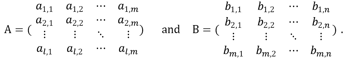
Matrix multiplication is an operation performed on two matrices, which preserves some of the structure and character of both matrices. Formally, suppose we are given two matrices , an matrix, and , an matrix, as follows:

The matrix product of and is an matrix whose -th entry is given by the following equation:

Note that the number of columns of the first matrix must match the number of rows of the second matrix in order for matrix multiplication to be defined. We usually write for the matrix product of and , if it is defined. Matrix multiplication is a peculiar operation. It is not commutative like most other arithmetic operations: even if and can both be computed, there is no need for them to be equal. In practice, this means that the order of multiplication matters for matrices. This arises from the origins of matrix algebras as representations of linear maps, where multiplication corresponds to the composition of functions.

Python has an operator reserved for matrix multiplication, @, which was added in Python 3.5. NumPy arrays implement the operator to perform matrix multiplication. Note that this is fundamentally different from the component-wise multiplication of arrays, *:

A = np.array([[1, 2], [3, 4]])
B = np.array([[-1, 1], [0, 1]])
A @ B
# array([[-1, 3],
#           [-3, 7]])
A * B # different from A @ B
# array([[-1, 2],
#           [ 0, 4]])

The identity matrix is a neutral element under matrix multiplication. That is, if is any matrix and is the identity matrix, then , and similarly, if is an matrix, then . This can be easily checked for specific examples using NumPy arrays:

A = np.array([[1, 2], [3, 4]])
I = np.eye(2)
A @ I
# array([[1., 2.],
#           [3., 4.]])

You can see that the printed resulting matrix is equal to the original matrix. The same is true if we reversed the order of and and performed the multiplication . In the next section, we’ll look at matrix inverses; a matrix that when multiplied by gives the identity matrix.

Determinants and inverses

The determinant of a square matrix is important in most applications because of its strong link with finding the inverse of a matrix. A matrix is square if the number of rows and columns are equal. In particular, a matrix that has a nonzero determinant has a (unique) inverse, which translates to unique solutions of certain systems of equations. The determinant of a matrix is defined recursively. Suppose that we have a generic matrix, as follows:

The determinant of this generic matrix is defined by the following formula:

For a general matrix where , we define the determinant recursively. For , the --th submatrix is the result of deleting the th row and th column from . The submatrix is an matrix, and so we can compute the determinant. We then define the determinant of to be the following quantity:

In fact, the index 1 that appears in the preceding equation can be replaced by any and the result will be the same.

The NumPy routine for computing the determinant of a matrix is contained in a separate module called linalg. This module contains many common routines for linear algebra, which is the branch of mathematics that covers vector and matrix algebra. The routine for computing the determinant of a square matrix is the det routine:

from numpy import linalg
linalg.det(A)  # -2.0000000000000004

Note that a floating-point rounding error has occurred in the calculation of the determinant.

The SciPy package, if installed, also offers a linalg module, which extends NumPy’s linalg. The SciPy version not only includes additional routines, but it is also always compiled with BLAS and Linear Algebra PACKage (LAPACK) support, while for the NumPy version, this is optional. Thus, the SciPy variant may be preferable, depending on how NumPy was compiled, if speed is important.

The inverse of an matrix is the (necessarily unique) matrix , such that , where denotes the identity matrix and the multiplication performed here is matrix multiplication. Not every square matrix has an inverse; those that do not are sometimes called singular matrices. In fact, a matrix is non-singular (that is, has an inverse) if, and only if, the determinant of that matrix is not 0. When has an inverse, it is customary to denote it by .

The inv routine from the linalg module computes the inverse of a matrix if it exists:

linalg.inv(A)
# array([[-2. , 1. ],
#           [ 1.5, -0.5]])

We can check that the matrix given by the inv routine is indeed the matrix inverse of A by matrix multiplying (on either side) by the inverse and checking that we get the 2 × 2 identity matrix:

Ainv = linalg.inv(A)
Ainv @ A
# Approximately
# array([[1., 0.],
#           [0., 1.]])
A @ Ainv
# Approximately
# array([[1., 0.],
#           [0., 1.]])

There will be a floating-point error in these computations, which has been hidden away behind the Approximately comment, due to the way that matrix inverses are computed.

The linalg package also contains a number of other methods such as norm, which computes various norms of a matrix. It also contains functions for decomposing matrices in various ways and solving systems of equations.

There are also the matrix analogs of the exponential function expm, the logarithm logm, sine sinm, cosine cosm, and tangent tanm. Note that these functions are not the same as the standard exp, log, sin, cos, and tan functions in the base NumPy package, which apply the corresponding function on an element-by-element basis. In contrast, the matrix exponential function is defined using a power series of matrices:

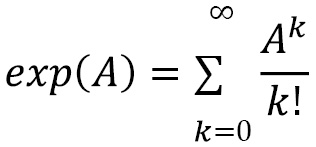
This is defined for any matrix , and denotes the th matrix power of ; that is, the matrix multiplied by itself times. Note that this “power series” always converges in an appropriate sense. By convention, we take , where is the identity matrix. This is completely analogous to the usual power series definition of the exponential function for real or complex numbers, but with matrices and matrix multiplication in place of numbers and (regular) multiplication. The other functions are defined in a similar fashion, but we will skip the details.

In the next section, we’ll see one area where matrices and their theory can be used to solve systems of equations.

Systems of equations

Solving systems of (linear) equations is one of the main motivations for studying matrices in mathematics. Problems of this type occur frequently in a variety of applications. We start with a system of linear equations written as follows:

Here, is at least two, and are known values, and the values are the unknown values that we wish to find.

Before we can solve such a system of equations, we need to convert the problem into a matrix equation. This is achieved by collecting together the coefficients into an matrix and using the properties of matrix multiplication to relate this matrix to the system of equations. So, we construct the following matrix containing the coefficients taken from the equations:

Then, if we take to be the unknown (column) vector containing the values and to be the (column) vector containing the known values , then we can rewrite the system of equations as the following single matrix equation:

We can now solve this matrix equation using matrix techniques. In this situation, we view a column vector as an matrix, so the multiplication in the preceding equation is matrix multiplication. To solve this matrix equation, we use the solve routine in the linalg module. To illustrate the technique, we will solve the following system of equations as an example:

These equations have three unknown values: , , and . First, we create a matrix of coefficients and the vector . Since we are using NumPy as our means of working with matrices and vectors, we create a two-dimensional NumPy array for the matrix and a one-dimensional array for :

import numpy as np
from numpy import linalg
A = np.array([[3, -2, 1], [1, 1, -2], [-3, -2, 1]])
b = np.array([7, -4, 1])

Now, the solution to the system of equations can be found using the solve routine:

linalg.solve(A, b)  # array([ 1., -1., 2.])

This is indeed the solution to the system of equations, which can be easily verified by computing A @ x and checking the result against the b array. There may be a floating-point rounding error in this computation.

The solve function expects two inputs, which are the matrix of coefficients and the right-hand side vector . It solves the system of equations using routines that decompose matrix into simpler matrices to quickly reduce to an easier problem that can be solved by simple substitution. This technique for solving matrix equations is extremely powerful and efficient and is less prone to the floating-point rounding errors that dog some other methods. For instance, the solution to a system of equations could be computed by multiplying (on the left) by the inverse of the matrix , if the inverse is known. However, this is generally not as good as using the solve routine since it may be slower or result in larger numerical errors.

In the example we used, the coefficient matrix was square. That is, there is the same number of equations as there are unknown values. In this case, the system of equations has a unique solution if (and only if) the determinant of this matrix is not . In cases where the determinant of is , one of two things can happen: the system can have no solution, in which case we say that the system is inconsistent, or there can be infinitely many solutions. The difference between a consistent and inconsistent system is usually determined by the vector . For example, consider the following systems of equations:

The left-hand system of equations is consistent and has infinitely many solutions; for instance, taking and or and are both solutions. The right-hand system of equations is inconsistent, and there are no solutions. In both of the preceding systems of equations, the solve routine will fail because the coefficient matrix is singular.

The coefficient matrix does not need to be square for the system to be solvable—for example, if there are more equations than there are unknown values (a coefficient matrix has more rows than columns). Such a system is said to be over-specified and, provided that it is consistent, it will have a solution. If there are fewer equations than there are unknown values, then the system is said to be under-specified. Under-specified systems of equations generally have infinitely many solutions if they are consistent since there is not enough information to uniquely specify all the unknown values. Unfortunately, the solve routine will not be able to find solutions for systems where the coefficient matrix is not square, even if the system does have a solution.

In the next section, we’ll discuss eigenvalues and eigenvectors, which arise by looking at a very specific kind of matrix equation, similar to those seen previously.

Eigenvalues and eigenvectors

Consider the matrix equation , where is a square () matrix, is a vector, and is a number. Numbers for which there is an that solves this equation are called eigenvalues, and the corresponding vectors are called eigenvectors. Pairs of eigenvalues and corresponding eigenvectors encode information about the matrix , and are therefore important in many applications where matrices appear.

We will demonstrate computing eigenvalues and eigenvectors using the following matrix:

We must first define this as a NumPy array:

import numpy as np
from numpy import linalg
A = np.array([[3, -1, 4], [-1, 0, -1], [4, -1, 2]])

The eig routine in the linalg module is used to find the eigenvalues and eigenvectors of a square matrix. This routine returns a pair (v, B), where v is a one-dimensional array containing the eigenvalues and B is a two-dimensional array whose columns are the corresponding eigenvectors:

v, B = linalg.eig(A)

It is perfectly possible for a matrix with only real entries to have complex eigenvalues and eigenvectors. For this reason, the return type of the eig routine will sometimes be a complex number type such as complex32 or complex64. In some applications, complex eigenvalues have a special meaning, while in others we only consider the real eigenvalues.

We can extract an eigenvalue/eigenvector pair from the output of eig using the following sequence:

i = 0 # first eigenvalue/eigenvector pair
lambda0 = v[i]
print(lambda0)
# 6.823156164525971
x0 = B[:, i] # ith column of B
print(x0)
# [ 0.73271846, -0.20260301, 0.649672352]

The eigenvectors returned by the eig routine are normalized so that they have norm (length) 1. (The Euclidean norm is defined to be the square root of the sum of the squares of the members of the array.) We can check that this is the case by evaluating in the norm of the vector using the norm routine from linalg:

linalg.norm(x0)  # 1.0  - eigenvectors are normalized.

Finally, we can check that these values do indeed satisfy the definition of an eigenvalue/eigenvector pair by computing the product A @ x0 and checking that, up to floating-point precision, this is equal to lambda0*x0:

lhs = A @ x0
rhs = lambda0*x0
linalg.norm(lhs - rhs)  # 2.8435583831733384e-15 - very small.

The norm computed here represents the distance between the left-hand side (lhs) and the right-hand side (rhs) of the equation . Since this distance is extremely small (0 to 14 decimal places), we can be fairly confident that they are actually the same. The fact that this is not zero is likely due to floating-point precision error.

The theoretical procedure for finding eigenvalues and eigenvectors is to first find the eigenvalues by solving the following equation:

Here, is the appropriate identity matrix. The equation determined by the left-hand side is a polynomial in and is called the characteristic polynomial of . The eigenvector corresponding to the eigenvalue can then be found by solving the following matrix equation:

In practice, this process is somewhat inefficient, and there are alternative strategies for computing eigenvalues and eigenvectors numerically more efficiently.

We can only compute eigenvalues and eigenvectors for square matrices; for non-square matrices, the definition does not make sense. There is a generalization of eigenvalues and eigenvectors to non-square matrices called singular values. The trade-off that we have to make in order to do this is that we must compute two vectors and , and a singular value that solves the following equation:

If is an matrix, then will have elements and will have elements. The interesting vectors are actually the (orthonormal) eigenvectors of the symmetric matrix with the eigenvalue . From these values, we can find the vectors using the previous defining equation. This will generate all of the interesting combinations, but there are additional vectors and where and .

The utility of singular values (and vectors) comes from the singular value decomposition (SVD), which writes the matrix as a product:

Here, has orthogonal columns and has orthogonal rows, and is a diagonal matrix, usually written so that the values decrease as one moves along the leading diagonal. We can write this formula out in a slightly different way, as follows:

What this says is that any matrix can be decomposed into a weight sum of outer products—pretend and are matrices with rows and column and matrix multiply with the transpose of – of vectors.

Once we have performed this decomposition, we can look for values that are especially small, which contribute very little to the value of the matrix. If we throw away the terms with small values, then we can effectively approximate the original matrix by a simpler representation. This technique is used in principal component analysis (PCA)—for example, to reduce a complex, high-dimensional dataset to a few components that contribute the most to the overall character of the data.

In Python, we can use the linalg.svd function to compute the SVD of a matrix. This works in a similar way to the eig routine described previously, except it returns the three components of the decomposition:

mat = np.array([[0., 1., 2., 3.], [4., 5., 6., 7.]])
U, s, VT = np.linalg.svd(mat)

The arrays returned from this function have shapes (2, 2), (2,), and (4, 4), respectively. As the names suggest, the U matrix and VT matrices are those that appear in the decomposition, and s is a one-dimensional vector containing the nonzero singular values. We can check that decomposition is correct by reconstructing the matrix and evaluating the product of the three matrices:

Sigma = np.zeros(mat.shape)
Sigma[:len(s), :len(s)] = np.diag(s)
# array([[11.73352876, 0., 0., 0.],
#        [0., 1.52456641, 0.,  0.]])
reconstructed = U @ Sigma @ VT
# array([[-1.87949788e-15, 1., 2., 3.],
#           [4., 5., 6., 7.]])

Notice that the matrix has been reconstructed almost exactly, except for the first entry. The value in the top-left entry is very close to zero—within floating point error—so can be considered zero.

Our method for constructing the matrix is rather inconvenient. The SciPy version of the linalg module contains a special routine for reconstructing this matrix from the one-dimensional array of singular values called linalg.diagsvd. This routine takes the array of singular values, s, and the shape of the original matrix and constructs the matrix with the appropriate shape:

Sigma = sp.linalg.diagsvd(s, *mat.shape)

(Recall that the SciPy package is imported under the alias sp.) Now, let’s change pace and look at how we might be more efficient in the way we describe matrices in which most of the entries are zero. These are the so-called sparse matrices.

Sparse matrices

Systems of linear equations such as those discussed earlier are extremely common throughout mathematics and, in particular, in mathematical computing. In many applications, the coefficient matrix will be extremely large, with thousands of rows and columns, and will likely be obtained from an alternative source rather than simply entering by hand. In many cases, it will also be a sparse matrix, where most of the entries are 0.

A matrix is sparse if a large number of its elements are zero. The exact number of elements that need to be zero in order to call a matrix sparse is not well defined. Sparse matrices can be represented more efficiently—for example, by simply storing the indexes and the values that are nonzero. There are entire collections of algorithms for sparse matrices that offer great improvements in performance, assuming the matrix is indeed sufficiently sparse.

Sparse matrices appear in many applications, and often follow some kind of pattern. In particular, several techniques for solving partial differential equations (PDEs) involve solving sparse matrix equations (see Chapter 3, Calculus and Differential Equations), and matrices associated with networks are often sparse. There are additional routines for sparse matrices associated with networks (graphs) contained in the sparse.csgraph module. We will discuss these further in Chapter 5, Working with Trees and Networks.

The sparse module contains several different classes representing the different means of storing a sparse matrix. The most basic means of storing a sparse matrix is to store three arrays, two containing integers representing the indices of nonzero elements, and the third the data of the corresponding element. This is the format of the coo_matrix class. Then, there are the compressed sparse column (CSC) (csc_matrix) and the compressed sparse row (CSR) (csr_matrix) formats, which provide efficient column or row slicing, respectively. There are three additional sparse matrix classes in sparse, including dia_matrix, which efficiently stores matrices where the nonzero entries appear along a diagonal band.

The sparse module from SciPy contains routines for creating and working with sparse matrices. We import the sparse module from SciPy using the following import statement:

import numpy as np
from scipy import sparse

A sparse matrix can be created from a full (dense) matrix or some other kind of data structure. This is done using the constructor for the specific format in which you wish to store the sparse matrix.

For example, we can take a dense matrix and store it in CSR format by using the following command:

A = np.array([[1., 0., 0.], [0., 1., 0.], [0., 0., 1.]])
sp_A = sparse.csr_matrix(A)
print(sp_A)
#  (0, 0)  1.0
#  (1, 1)  1.0
#  (2, 2)  1.0

If you are generating a sparse matrix by hand, the matrix probably follows some kind of pattern, such as the following tridiagonal matrix:

Here, the nonzero entries appear on the diagonal and on either side of the diagonal, and the nonzero entries in each row follow the same pattern. To create such a matrix, we could use one of the array creation routines in sparse such as diags, which is a convenience routine for creating matrices with diagonal patterns:

T = sparse.diags([-1, 2, -1], (-1, 0, 1),   
    shape=(5, 5), format="csr")

This will create a matrix , as described previously, and store it as a sparse matrix in CSR format. The first argument specifies the values that should appear in the output matrix, and the second argument is the positions relative to the diagonal position in which the values should be placed. So, the 0 index in the tuple represents the diagonal entry, -1 is to the left of the diagonal in the row, and +1 is to the right of the diagonal in the row. The shape keyword argument gives the dimensions of the matrix produced, and the format specifies the storage format for the matrix. If no format is provided using the optional argument, then a reasonable default will be used. The array T can be expanded to a full (dense) matrix using the toarray method:

T.toarray()
# array([[ 2, -1,  0,  0,  0],
#           [-1,  2, -1,  0,  0],
#           [ 0, -1,  2, -1,  0],
#           [ 0,  0, -1,  2, -1],
#           [ 0,  0,  0, -1,  2]])

When the matrix is small (as it is here), there is little difference in performance between the sparse solving routine and the usual solving routines.

Once a matrix is stored in a sparse format, we can use the sparse solving routines in the linalg submodule of sparse. For example, we can solve a matrix equation using the spsolve routine from this module. The spsolve routine will convert the matrix into CSR or CSC, which may add additional time to the computation if it is not provided in one of these formats:

from scipy.sparse import linalg
linalg.spsolve(T.tocsr(), np.array([1, 2, 3, 4, 5]))
# array([ 5.83333333, 10.66666667, 13.5 , 13.33333333, 9.16666667])

The sparse.linalg module also contains many of the routines that can be found in the linalg module of NumPy (or SciPy) that accept sparse matrices instead of full NumPy arrays, such as eig and inv.

This concludes our tour of the basic tools for mathematics available in Python and its ecosystem. Let’s summarize what we’ve seen.

Summary

Python offers built-in support for mathematics with some basic numerical types, arithmetic, extended precision numbers, rational numbers, complex numbers, and a variety of basic mathematical functions. However, for more serious computations involving large arrays of numerical values, you should use the NumPy and SciPy packages. NumPy provides high-performance array types and basic routines, while SciPy provides more specific tools for solving equations and working with sparse matrices (among many other things).

NumPy arrays can be multi-dimensional. Two-dimensional arrays have matrix properties that can be accessed using the linalg module from either NumPy or SciPy (the former is a subset of the latter). Moreover, there is a special operator in Python for matrix multiplication, @, which is implemented for NumPy arrays. SciPy also provides support for sparse matrices via the sparse module. We also touched on matrix theory and linear algebra, which underpins most of the numerical methods found in this book—often behind the scenes.

In the next chapter, we’ll get started looking at some recipes.

Further reading

There are many mathematical textbooks describing the basic properties of matrices and linear algebra, which is the study of vectors and matrices. The following are good introductory texts for linear algebra:

• Strang, G. (2016). Introduction to Linear Algebra. Wellesley, MA: Wellesley-Cambridge Press, Fifth Edition.
• Blyth, T. and Robertson, E. (2013). Basic Linear Algebra. London: Springer London, Limited.

NumPy and SciPy are part of the Python mathematical and scientific computing ecosystem and have extensive documentation that can be accessed from the official website, https://scipy.org. We will see several other packages from this ecosystem throughout this book.

More information about the BLAS and LAPACK libraries that NumPy and SciPy use behind the scenes can be found at the following links:

• BLAS: https://www.netlib.org/blas/
• LAPACK: https://www.netlib.org/lapack/