
8
Application of Integer Programming in Allocating Energy Resources in Rural Africa
Elias Munapo
Department of Statistics and Operations Research, School of Economic Sciences, North West University, Mahikeng, South Africa
8.1 Introduction
The quadratic assignment problem (QAP) can be defined as the problem whereby a set of facilities are allocated to a set of locations in such a way that the cost is a function of the distance and flow between the facilities. In this problem, the costs are associated with a facility being placed at a certain location. The objective is to minimize the assignment of each facility to a location. To date, the QAP has been believed to be very difficult, and heuristics were believed to be the methods of choice as given in Munapo [1]. Various heuristics have been developed, for example, Hahn and Grant [2], Ramakrishnan et al. [3], and Drezner [4]. For more developments in solving QAP, you may see Mohamed et al. [5], Adams and Johnson [6], Cela [7], Nagarajan and Sviridenko [8], Rego et al. [9], Xia [10] and Yang et al. [11].
8.1.1 Applications of the QAP
In addition to allocating resources and having importance in decision fame work, the QAP can also be used in numerical analysis, dartboard construction, archaeology, statistical analysis, reaction chemistry, economic problem modeling, hospital lay‐out, backboard wiring problem, and campus planning model. These are briefly explained as follows.
- Numerical analysis. The QAP can be used to generate initial permutations for the least‐squares unidimensional scaling of symmetric proximity matrices. This method is used in numerical analysis.
- Dartboard construction. A dart game is a game played by throwing darts at a circular board with numbered spaces. The problem of locating the numbers around a dartboard optimally can be formulated as a QAP. The same problem can also be modeled as a traveling salesman problem.
- Chemical reactions. In some chemical reactions, some chemical processes and complexes can be modeled as a QAP. The solution to this problem can be modeled as a QAP, and its optimal solution gives the optimal chemical process or optimal chemical reaction.
- Computer backboard wiring. The objective of computer backboard wiring is to minimize the total length of wiring used for the interconnection of components. A backboard is made of electronic components which require wiring. If the wiring is minimized, we save wiring costs and an improved computational time.
- Archaeology. In archaeology, various forms of data can be collected from all angles of archeology. There are also so many ways that are used to analyze these forms of data. Qualitative, quantitative, and mixed methods are some of these ways. In addition, various types of these data forms can be expressed as mathematical or economic models. The QAP is one such economic model.
- Hospital Layout. This problem comprises of assigning locations or departments to facilities or clinics in a way that minimizes the total distance that is traveled by patients. Some important factors such as human and economic factors are considered when planning a hospital.
8.2 Quadratic Assignment Problem Formulation
There are so many mathematical formulations for QAP. In this paper, we use the linear form proposed by Munapo in 2012 [1]. This linear form is an extension of the formulation introduced by Koopmans and Beckmann in 1957 [12]. In this formulation, we assume that new buildings are to be placed on a piece of land and n sites have been identified as sites for the buildings. We also assume that each building has a special function.
8.2.1 Koopmans–Beckmann Formulation
Let
- aij be the walking distance between sites i and j.
- bkl be the number of people per week who circulate between buildings k and l.
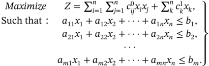
Then, the Koopmans–Beckmann formulation of the QAP is given as follows:

In this formula, there are n2 variables and 2n constraints [12].
8.3 Current Linearization Technique
The current technique can linearize the Koopmans–Beckmann model to the form given in (8.2).

Solving this, linearized QAP model becomes very difficult as n increases in size. This linearized model has (n4 + n2) variables and O(n4) constraints. This is very difficult to manage as n becomes large.
8.3.1 The General Quadratic Binary Problem
The Koopmans–Beckmann is a special case of a quadratic binary problem.
Let a general case of the quadratic binary problem be represented in (8.3a).
where
 and
and  are constants,
  ,
,
Budgetary constraints are given in (8.3b).
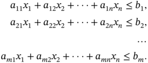
The budgetary constraints give the amounts that are available for the construction of the gas fuel site. These constraints also give the minimum amount of money that is required for the fuel gas sites. These constraints depend on a country.
In this case, there are n cites. The total distance traveled by people around the site is given as the coefficient of that site or combined sites.
This model has application in the allocation of gas stations in rural African villages. Most African governments are now banning the use of firewood as a measure to curb deforestation. People in these areas are being asked to use gas stoves and there is a need to make the fuel gas available to these remote villages. The problem of locating the fuel gas stations in rural areas in such a way that the total distance traveled by the villagers is minimized can be modeled as a QAP. The QAP is given in 8.3a. In this model, the optimal solution gives the minimal total distance traveled by all the villagers to get fuel gas. In developing this model, paths giving the shortest distance to these fuel stations are used. People walk or use bicycles or donkeys on these shortest paths, and it may not be possible with cars. People with cars use the long winding road to access these fuel gas stations. In addition to shortest paths, village or area populations are used in the modeling process. The coefficient of a variable or product of variables gives the average total distance traveled around a site or two sites.
The variables xixj where i = j.
If i = j then ![]() . For binary integer variables, we have the following.
. For binary integer variables, we have the following.

Thus ![]() can be replaced by xi in the objective function. Similarly,
can be replaced by xi in the objective function. Similarly, ![]() can also be replaced by xj in the objective function. Note that this substitution on its own does not change the number of variables in the problem.
can also be replaced by xj in the objective function. Note that this substitution on its own does not change the number of variables in the problem.
The variables xixj where i ≠ j.
If i ≠ j then in the worst case there are ![]() combinations of such variables in the objective function.
combinations of such variables in the objective function.
Justification: Suppose that we have:
- Two variables. (x1 and x2) then in the worst case we can have x1x2 as the only possible combination of variables.
- Three variables. (x1x2 and x3) then in the worst case we can have x1x2, x1x3 and x2x3 as the possible combinations of variables. Thus these three variables give 3 possible combinations.
- n variables. (x1, x2, …, xn − 1 and xn) then in the worst case we can have x1x2, x1x3, …, x1xn, x2x3, x2x4, …, x2xn, …, xn − 1xn as the possible combinations. The n variables give
 possible combinations.
8.3.2 Linearizing the Quadratic Binary Problem
The variable combinations xixj where i ≠ j must be removed in order to make the objective function linear. This is done by using the following substitution.
8.3.2.1 Variable Substitution
Let
where δr is also a binary variable and ![]() .
.
Such that:

8.3.2.2 Justification
We have to show that the solution space Ω(xixj) = {0, 1) is also the solution space for Ω(δr), every point in Ω(xixj) has a corresponding point in Ω(δr) and that xixj = δr for all corresponding points.
Solution Space for xixj i.e. Ω(xixj)

Solution Space for δr i.e. Ω(δr)

Corresponding Points
| Point in Ω(xixj) | Corresponding point in Ω(δr) |
|---|---|
8.3.3 Number of Variables and Constraints in the Linearized Model
Two extra variables are added to every product of variables xixj where i ≠ j, that appear in the objective function. In the general case of the quadratic binary problem, there are ![]() products as shown in Section 8.2. Thus there are
products as shown in Section 8.2. Thus there are
This gives a total of n(n − 1) new variables + n original variables = n2 variables.
Also two extra constraints are added for every product of variables xixj where i ≠ jthat appears in the objective function. The total number of new constraints is given by (8.8).
The total number constraints ![]() is given by,
is given by,

8.3.4 Linearized Quadratic Binary Problem
Then linearized model becomes as given in (8.10).


8.3.5 Reducing the Number of Extra Constraints in the Linear Model
As n becomes large, solving a linear model with n(n − 1) extra constraints increases in complexity. The number of extra constraints can be reduced by half. The following constraints can be combined into one.

The first constraint can be expressed as given in (8.11,8.12).
Since ![]() cannot exceed one as given in (8.13),
cannot exceed one as given in (8.13),
This reduces the number of extra constraints and variables to ![]()
8.3.6 The General Binary Linear (BLP) Model
Let any BLP model be represented by (8.14).
Minimize CXT,

8.3.6.1 Convex Quadratic Programming Model
Let a quadratic programming problem be represented by (8.15).
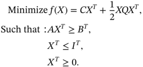
where  .
.
We assume that:
- (i) matrix Q is symmetric and positive definite,
- (ii) function f(X) is strictly convex,
- (iii) since constraints are linear, the solution space is convex,
- (iv) any maximization quadratic problem can be changed into a minimization and vice versa.
If f(X) is strictly convex for all points in the convex region, the local minimum is also the global minimum of the quadratic problem [13].
8.3.6.2 Transforming Binary Linear Programming (BLP) Into a Convex/Concave Quadratic Programming Problem
Let ![]()
Such that: XT + ST = IT and ST ≥ 0.
The convex quadratic objective function then becomes as given in (8.17).

In matrix form, it simplifies to (8.18).
The BLP becomes the convex quadratic problem given in (8.19).

where ℓ1 and ℓ2 are very large in terms of their sizes compared to any of the coefficients in the objective function. For this to work, the following must be satisfied.
Note that the weights of 1 000 and 1 000 000 depend on the sizes of the coefficients of the problem. For some small binary linear problems with small coefficients, weights of 10 and 1000 can be used effectively.
Enforcer ℓ2(x1s1 + x2s2 + ⋯ + xnsn).
Since this is a minimization quadratic objective function, the objective function will be minimal when (8.23) is satisfied.
This is possible when either xj = 0 or sj = 0. Munapo [14] termed the expression in (8.23) an enforcer since it forces the variables to assume only binary values.
8.3.6.3 Equivalence
The two quantities are equal if xj = 0 or xj = 1.
Similarly the two quantities are equal if sj = 0 or sj = 1.
Convexity of ![]() Since
Since ![]() , then this function
, then this function ![]() is convex if and only if it has second‐order partial derivatives for each point
is convex if and only if it has second‐order partial derivatives for each point ![]() and for each
and for each ![]() , all principal minors of the Hessian matrix are none negative.
, all principal minors of the Hessian matrix are none negative.
Proof
In this case

This has continuous second‐order partial derivatives and the 2n by 2n Hessian matrix is given by (8.27).
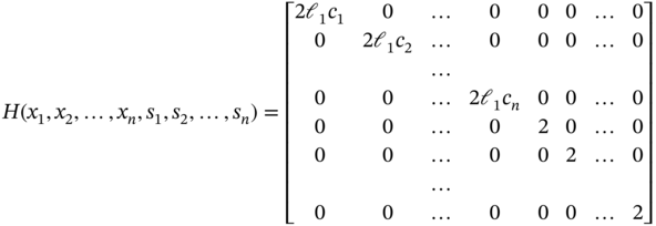
Since all principal minors of H(x1, x2, …, xn, s1, s2, …, sn) are non‐negative, f(x1, x2, …, xn, s1, s2, …, sn) is convex. See [14] for more on convex functions.
Note that ![]() . Thus the matrix H is symmetric and positive definite.
. Thus the matrix H is symmetric and positive definite.
The binary solution that minimizes ![]() also minimizes c1x1 + c2x2 + ⋯ + cnxn
also minimizes c1x1 + c2x2 + ⋯ + cnxn
From ![]() , ℓ2 is very large and ℓ1 < < ℓ2 then ℓ2(x1s1 + x2s2 + ⋯ + xnsn) = 0.
, ℓ2 is very large and ℓ1 < < ℓ2 then ℓ2(x1s1 + x2s2 + ⋯ + xnsn) = 0.
This is the same as just, minimize ![]() .
.
This reduces to, minimize c1x1 + c2x2 + ⋯ + cnxn.
8.4 Algorithm
The procedure is summarized in the following steps.
- Step 1: Linearize the QAP to a binary linear problem
- Step 2: Convert binary linear problem into a convex quadratic programming problem
- Step 3: Use an interior point algorithm to solve the convex quadratic programming problem
Numerical illustration (This is a QAP for locating fuel gas stations to four possible sites)
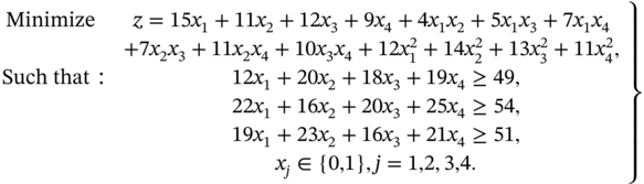
There are four possible sites for fuel gas stations for this problem. The optimal solution to (8.28) gives the minimum total distance that can be traveled by the villagers to obtain fuel gas.
In this case, the three budgetary constraints give the minimum amounts of money required to open the gas sites in terms of thousands of SA rands.
8.4.1 Making the Model Linear
Using ![]() and xixj = δr, the linear model in the numerical illustration becomes as given in (8.29).
and xixj = δr, the linear model in the numerical illustration becomes as given in (8.29).

where δi ∈ {0, 1}, i = 1, 2, 3, 4, 5, 6. This formulation was proposed by Munapo [1].
Changing the problem into a convex quadratic problem

where si ∈ {0, 1}, i = 1, 2, 3, 4, 5, 6 and ![]() .
.
Using ℓ1 = 1000(27 + 23 + 25 + 19 + 4 + 5 + 7 + 7 + 11 + 10) = 138 000 and ℓ2 = 1 000 000(27 + 23 + 25 + 19 + 4 + 5 + 7 + 7 + 11 + 10) = 138 000 000. The optimal solution by the interior point algorithm becomes as given in (8.31).
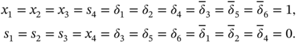
In terms of the original problem, opening fuel gas stations at sites 1, 2, and 3 will minimize the total distance traveled by all the villagers to obtain fuel gas.
8.5 Conclusions
The reason for converting the BLP into a convex quadratic programming model is to use the available efficient interior point algorithms which can solve convex quadratic problems in polynomial time. If the QAP which is NP‐hard can be converted into a convex quadratic problem which can be solved in polynomial time then P=NP. This implies that the QAP is not NP‐hard. In the future, we will consider increasing the complexity of the problem by making multi‐objective/multi‐level/variables with uncertainty (i.e. stochastic or fuzzy applications). In addition, when people visit a site, they do that with the intention of doing more than one thing, i.e. getting the gas and going to the grinding mill and/or visiting a clinic. This is not easy to factor this additional task in the nonlinear objective function of the QAP. Efforts will be made in the future to incorporate this additional task into single or multi‐objective quadratic assignment model which may be stochastic or fuzzy.
References
- 1 Munapo, E. (2012). Reducing the number of new constraints and variables in a linearised quadratic assignment problem. African Journal of Agricultural Research 2 (29): 3147–3152.
- 2 Hahn, P. and Grant, T. (2008). An algorithm for the generalized quadratic assignment problem. Computational Optimization and Applications 40 (3): 351–372.
- 3 Ramakrishnan, K., Resende, M. et al. (2002). Tight QAP bounds via linear programming. In: Combinatorial and Global Optimization (ed. P. Pardalos, A. Migdalas and R. Burkard), 297–303. Singapore: World Scientific Publishing.
- 4 Drezner, Z. (2008). Extensive experiments with hybrid genetic algorithms for the solution of the quadratic assignment problem. Computers & Operations Research 35 (3): 717–736.
- 5 Mohamed Manogaran, A.‐B., Rashad, G., Zaied, H., and Nasser, A. (2018). A comprehensive review of quadratic assignment problem: variants, hybrids and applications. Journal of Ambient Intelligence and Humanized Computing 9 (5): 1–24. https://doi.org/10.1007/s12652-018-0917-x.
- 6 Adams, W.P. and Johnson, T.A. (1994). Improved linear programming‐based lower bounds for the quadratic assignment problem. In: Quadratic Assignment and Related Problems, Volume 16 of DIMACS Series in Discrete Mathematics and Theoretical Computer Science, vol. 16 (ed. P.M. Pardalos and H. Wolkowicz), 43–75. AMS.
- 7 Cela, E. (1998). The quadratic assignment problem: theory and algorithms. In: Combinatorial Optimization. Dordrecht: Kluwer Academic Publishers.
- 8 Nagarajan, V. and Sviridenko, M. (2009). On the maximum quadratic assignment problem. Mathematics of Operations Research 34 (4): 859–868.
- 9 Rego, C., James, T., and Fred, G.F. (2010). An ejection chain algorithm for the quadratic assignment problem. Networks 56 (3): 188–206.
- 10 Xia, Y. (2010). An efficient continuation method for quadratic assignment problems. Computers and Operations Research 37 (6): 1027–1032.
- 11 Yang, X., Lu, Q., Li, C., and Liao, X. (2008). Biological computation of the solution to the quadratic assignment problem. Applied Mathematics and Computation 200 (1): 369–377.
- 12 Koopmans, T. and Beckmann, M. (1957). Assignment problems and the location of economic activities. IEEE Econometrica 25 (1): 53–76.
- 13 Munapo, E. (2020). The traveling salesman problem: network properties, convex quadratic formulation, and solution, Chap. 6. In: Research Advancements in Smart Technology, Optimization, and Renewable Energy, 88–109. IGI Global ISBN 9781799839705 (hardcover) | ISBN 9781799850397 (paperback) | ISBN 9781799839712 (ebook).
- 14 Munapo, E. (2016). Second Proof that N = NP, 5th Engineering Optical Conference, 19–23. Brazil: Iguassu Falls.