
13
Inventory Routing Problem with Fuzzy Demand and Deliveries with Priority
Paulina A. Avila‐Torres and Nancy M. Arratia‐Martinez
Universidad de las Américas Puebla, Department of Business Administration, Ex‐Hacienda Santa Catarina Mártir S/N, San Andrés Cholula, C.P., Puebla, 72810, México
13.1 Introduction
Since decades ago, one important challenge is to remain competitive. In order to achieve this, the logistic systems must be significantly improved, and the distribution of goods is the most expensive process. Consequently, making an optimal distribution plan will help to save on transportation costs [1]. Due to this, some authors like Campbell et al. [2] and Moin and Salhi [3] discussed the importance of integration of inventory management and transportation and how these two are interrelated. Yugang et al. [4] mention that the coordination of inventory and transportation decisions in multiple period is the key for the optimization of the inventory routing problem (IRP).
The IRP is an extension of the VRP that involves routing and inventory decisions [5]. In IRP, customers have to be served over a discrete‐time horizon by a fleet of capacitated vehicles starting and ending the routes at a depot [6]. Campbell et al. [2] mention the three decisions made in this kind of problem are: (i) When to serve a customer?, (ii) How much to deliver to a customer when it is served?, and (iii) Which delivery route to use?
IRP may be applied in several industries such as gas companies, petrochemicals, clothing, auto parts, etc. [3]. Over the years, many authors have worked in creating reviews of the IRP considering different characteristics. For example, Andersson et al. [7] presented a survey with an emphasis on industrial applications. Coelho et al. [8] presented a survey focused on methodological aspects of the problem, including variants, models, and algorithms. Archetti et al. [6] presented and compared different formulations of IRP and valid inequalities are also presented, considering discrete‐time horizons and a fleet of capacitated vehicles. More recently, Roldán et al. [9] presented a survey of problems dealing with the stochastic nature of demand and lead times, a factor they identified as critical in real life. Then, Malladi and Sowlati [10] presented a review but considering sustainable aspects in the IRP; they stated that more common objectives are waste management, returnable transport item management, waste prevention and reduction, and emission reduction.
Many authors have incorporated real‐life characteristics making the problem more complex. For example, Savelsbergh and Song [11] worked in limited product availabilities at facilities where customers cannot be served using out‐and‐back tours; they designed tours that cover huge geographic areas and developed a greedy algorithm combined with optimization‐based improvement techniques. Yugang et al. [4] studied a multiperiod deterministic IRP with split deliveries and a limited fleet size, they presented an approximate approach that can solve large instances using Lagrangian relaxation, the objective is to minimize the inventory holding cost and transportation cost. Yugang et al. [4] reported that the coordination of inventory and transportation decisions in multiple periods is the key for the optimization of the IRP. The Economic Model Predictive Control (EMPC) strategy proposed by Athanassios and Ganas [12] used a multi‐period deterministic model; this strategy captures all attributes of reverse logistics and inventory routing.
Solving instances with a large number of customers with exact methods is very difficult; that is why, some authors have implemented or developed heuristics to solve this kind of problem. For example, Bard and Nananukul [13] compared some heuristics for an IRP. They formulated a mixed‐integer program maximizing the net benefits, but optimal solutions were not met with exact methods; so, they developed a two‐step procedure that first decides the quantity to deliver and then defines the route. They assume that demand is deterministic, a finite planning horizon and a fleet of same capacity. Yugang et al. [4] studied a multiperiod deterministic IRP with split deliveries and a limited fleet size. They presented an approximate approach that can near optimally solve large instances using Lagrangian relaxation; the objective was to minimize the inventory holding cost and transportation cost. Vansteenwegen and Mateo [14] presented an iterated local search metaheuristic to solve a single‐vehicle cyclic IRP.
Other authors have worked with a pickup and delivery inventory routing problem. For example, Iassinovskaia et al. [15] worked on this kind of problems with time windows; for small instances, they present a mixed‐integer linear program, and to solve large instances, they proposed a metaheuristic. In this kind of problem, in addition to having transportation and inventory costs, they consider some costs related to the returnable transport items (RTIs). Archetti et al. [16] considered a specific class of this problem where a commodity was available at several origins and demanded at several destinations. They proposed a mathematical model with several valid inequalities. Naccache et al. [17] work in multi‐pickup and delivery problem, they also consider time windows, in their problem, they collect and deliver items requested by the customer and solve the problem with an exact method, also they implemented a heuristic.
Authors like Moin et al. [18] considered a many‐to‐one distribution network, which means they assumed N suppliers where each provides distinct product to an assembly plant. They considered deterministic demand but variable over time, inventory cost at the plant but not at the supplier, unlimited capacitated vehicles. To solve the problem, they used genetic algorithms. Coelho et al. [19] presented an exact method to solve several kinds of IRP as a single vehicle, multi‐vehicles, different inventory policies, same or different capacities of trucks, etc.
Some authors as Campbell et al. [2] mentioned that in real life, the IRP is stochastic and dynamic. Also, Roldán et al. [9] mentioned that in practical situations of IRP, demand and lead times are not deterministic and the processes of inventory control and distribution are the keys for the performance in supply chain. Solyali et al. [20] considered the stochastic demand and introduced a robust IRP where a supplier distributes a single product to multiple customers facing dynamic uncertain demands over a finite discrete time horizon. They propose two robust Mixed‐Integer Programming (MIP) formulations and a new MIP formulation for the deterministic problem with backlogging demand allowed. They developed a branch‐and‐cut algorithm using the proposed formulation. Bertazzi et al. [21] also considered stochastic demand and order‐up‐to level policy and proposed a hybrid rollout algorithm. Moin and Halim [22] considered an IRP with stochastic and dynamic demand modeled as a Markov decision process; a hybrid rollout algorithm where a MILP is also used, and an ant bee colony algorithm is implemented.
Other authors have also dealt with the stochastic nature of the IRP. For example, Niakan and Rahimi [23] presented a model for healthcare issues considering fuzzy demand and transportation, representing the uncertainty using triangular fuzzy numbers. Qamsari et al. [24] proposed a model for the IRP with fuzzy time windows considering customer satisfaction; they divided the customers into categories and gave them a priority for visiting them. They proposed a column generation technique in order to obtain an optimal solution. They represented the fuzzy time windows with trapezoidal fuzzy numbers. Also, Micheli and Mantella [25] incorporated the stochastic demand assuming that is normally distributed. Authors like [26] used the fuzzy methodology in urban transport planning, considering demand and waiting time as triangular fuzzy numbers; they implemented two fuzzy methods (k‐preference and second index of Yager) and compared the results obtained. As we can see, most of the authors considered stochastic demand and this becomes the problem even more complex.
The objective of this research is to formulate a mathematical model that creates the weekly plan according to the inventory level and the uncertain demand of customers using triangular fuzzy numbers and giving priority to some customers. The model will be applied in a case study. Some of the findings of this chapter are as follows: the solution time increases when the number of customers with priority is high, and the higher the security degree, the lower the total cost. The remaining chapter is organized as follows: the problem description is presented in Section 13.2, the mathematical formulation in Section 13.3, the results of computational experiments are discussed in Section 13.4, and finally, the conclusions and future work are presented in Section 13.5.
13.2 Problem Description
This chapter is inspired by a producer and distributor company of gases in the northern region of Mexico. These kinds of companies deliver products such as oxygen, nitrogen, and argon in different ways, for example, big trucks, small trucks, and trucks with cylinders (Figure 13.1).
Some decisions related to this particular business are as follows:
- Production: How much, where, and what time to produce in order to save energy cost.
- Assignment: Decide from which plant each customer is going to be served.
- Assignment: Decide how to manage the fleet (own trucks and subcontracted).
The current decision process has six main steps (see Figure 13.2). First, the company has a responsible team to plan all routes for different plants and products, each member of the team has been assigned a plant and a product, this is a daily plan. Second, as part of their job, every day they have to verify the level of inventory and the consumption of each customer assigned to them. Third, they decide which customers are to be included in the route for the next day, based on the inventory level and consumption, which can vary momentarily. Fourth, once they have chosen the customers to visit, they create manually the order in which to visit the customers. Fifth, when the route they are creating is for hospitals, then those customers have to be first in the route. Sixth, when they create the route, they also must consider the window time of product reception with the customer.

Figure 13.1 The north region of Mexico for distribution.

Figure 13.2 Current decision process.
There are two main characteristics in this research, one is uncertain demand and the other is to give priority to the customers who required oxygen. In the next example (Figure 13.3) we explain how a route changes when some customers must be served first. In Figure 13.3 there are four customers (1–4) and one depot (0). On the left side of Figure 13.3, there are no customers with priority, so the routes are 0 → 3 → 4 → 1 → 2 → 0 (blue line) and 0 → 3 → 4 → 2 → 0 (red line). Then, when we assigned priority (right side of figure) to customers 1 and 2, the routes change. We first create an exclusive route for customer 2 (0 → 2 → 0, blue line), and then simultaneously create a second route to visit the other customers (0 → 3 → 4 → 0, blue line), in the second period the model creates a route to visit customers with a low inventory level (0 → 1 → 4 → 0, red line).
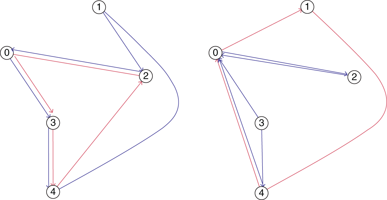
Figure 13.3 Example of the route both with and without priority.
In order to deal with demand uncertainty, we use fuzzy linear programming. In the following, we assume triangular fuzzy numbers, which, in general, will be denoted by ![]() where
where ![]() and
and ![]() denote the lower and upper limits, respectively, of the support of a fuzzy number
denote the lower and upper limits, respectively, of the support of a fuzzy number ![]() [27].
[27].
Here, we implement the approach of Adamo [28]. This method evaluates the fuzzy number based on the rightmost point of the ∝− cut given for a given ∝ [29]. Let us denote ![]() the fuzzy relation so determined. We impose the corresponding utility function to be an increasing function in the following particular sense [28]:
the fuzzy relation so determined. We impose the corresponding utility function to be an increasing function in the following particular sense [28]:
For any v1 ∈ Hv, v2 ∈ Hv,
where,
Given this property, any crisp utility function uα derived from ![]() and defined by
and defined by ![]() is an increasing function.
is an increasing function.
Brunelli and Mezei [29] mentioned that the approach of Adamo is the only one that satisfies all properties for ordering fuzzy numbers. They summarized the Adamo approach as follows:
where ∝ ∈ [0, 1] and ![]() . By definition, all the α‐cuts of fuzzy numbers are intervals; therefore, one can conveniently define them by means of their endpoints [29].
. By definition, all the α‐cuts of fuzzy numbers are intervals; therefore, one can conveniently define them by means of their endpoints [29].
13.3 Mathematical Formulation
The mathematical model presented in this section is based on Archetti et al. [30] and Archetti et al. [6] formulations.
We consider a directed network where the product is shipped from a depot to a set of customers (N′) over a time horizon T. Also, we consider that in t = 0, distribution and consumption of product do not exist.
The objective function (Eq. (13.1)) minimizes the inventory cost at depot (h0). I0t represents the inventory level at the depot for each period t, the objective function also minimizes the inventory cost at customers. (hi), and Iit indicates the inventory level at customer i for each period t and also minimizes the distribution cost cij from node i to node j, where the binary decision variable ![]() is equal to 1 if customer j is visited from customer i in the route k at the time t.
is equal to 1 if customer j is visited from customer i in the route k at the time t.
Constraint (13.2) is about the inventory level at the depot in the current period I0t that is equal to the inventory level at the depot in the previous period I0t − 1 plus the product available at the depot at the current period r0t plus the total product delivered to all customers ![]() at the current period t in the route k.
at the current period t in the route k.
Inventory level at customers (Iit) is represented with constraint (13.3); the inventory level at period t is equal to the inventory level the customer had at the previous period Iit − 1 minus the consumption of the product at the current period rit plus the total product delivered to the customer at the current period with any route ![]() . This inventory level can be represented as in the following constraint (13.3).
. This inventory level can be represented as in the following constraint (13.3).
In order to guarantee the correct operation of the tank, the inventory level at the customer must be greater or equal to a minimum inventory level, ![]() as expressed in constraint (13.4).
as expressed in constraint (13.4).
The constraints (13.5–13.7) are related to the order‐up‐to‐level policy. Constraints (13.5–13.6) indicate that the quantity delivered to the customer ![]() must be greater than or equal to the difference between the maximum capacity of the tank Ui and the inventory level at the previous period Iit − 1 but only if the customer was visited
must be greater than or equal to the difference between the maximum capacity of the tank Ui and the inventory level at the previous period Iit − 1 but only if the customer was visited ![]() in period t on route k. According to constraint (13.7), the quantity delivered to the customer
in period t on route k. According to constraint (13.7), the quantity delivered to the customer ![]() has to be less or equal than tank capacity Ui if the customer was visited
has to be less or equal than tank capacity Ui if the customer was visited ![]() .
.
Constraint (13.8) guarantees that the truck capacity (Q) will not be exceeded.
Each customer will be visited just by one truck as expressed in constraint (13.9).
The flow constraint (13.10) indicates that if the customer was visited, then for every arc entering to a customer, there must be one arc leaving the same customer.
The sub‐tour elimination constraint is represented in constraint (13.11) where E(S) is the set of all possible sub tours.
Constraint (13.12) allocates routes at the beginning to customers with priority deliveries (Pj).
The non‐negativity and integrality of variables are represented with constraints (13.13–13.15)
Also, the valid inequalities proposed by Archetti et al. [30] were implemented in the current framework.
13.4 Computational Experiments
First, a brief computational experiment was carried out with the main objective to study the effect on solution time when we add the priority rules that are part of this problem and the simple way, that means without considering uncertainty on demand.
Three groups of five instances with 5, 10, and 15 customers, respectively, were generated based on Archetti et al. [30] instances. All groups were created with different levels (0%, 25%, 50%, and 75% of customers) of priority.
The lineal mathematical model was implemented with ILOG CPLEX Optimization Studio version 12.8. The problem has a total of |N|^2 * (1+|K|*|T|) + 2(|N−1|*|T|*|K| variables. The time of solution is shown in Figure 13.4. In Figure 13.4a the solution time for the instances with 5 customers is presented, as you can see the solution time is very small, with less than a second. In this case, the solution time in instances with 0.25 fraction of the customers with priority takes more time, but still remains insignificant.

Figure 13.4 Solving time for instances with 5, 10, and 15 customers and different levels of priority (0, 0.25, 0.5, 0.75). (a) Solving time for instances with 5 customers. (b) Solving time for instances with 10 customers. (c) Solving time for instances with 15 customers.
In Figure 13.4b,c, the solution time of instances with 5 and 10 customers, respectively, are presented, the average time of solution for instances with 0.25 and 0.50 as a fraction of priority are smaller than those without any priority.
13.4.1 Numerical Example
In order to have a better understanding of the IRP problem and the application of the mathematical model elaborated in the previous section, we provide a semi‐real numerical example. First, we solve the case under certainty and then show the results when uncertainty exists.
To apply the mathematical model we first recollect the data about the consumers. Then, we get the driving distance between each pair of customers through google.com services. After the driving distance was reached, we established the inventory levels, the product consumption rate, and the complete data. Finally, the mathematical model was solved through the branch and bound algorithm in ILOG CPLEX Optimization Studio 12.8.
So, let us define a set of 14 consumers from two sectors, namely industry and health. The customer locations were recollected from real locations (open data) of the metropolitan region of Nuevo León, México. The locations are represented in Figure 13.5. The blue nodes are consumers in the industry sector and the red nodes are consumers in the health sector. We selected randomly a location to be depot location. According to the implementation in the software, this case has 1,883 variables and 806,782 constraints.

Figure 13.5 Locations of the consumers.
In Table 13.1, the complete data of the 14 customers are presented. In the first column, we assigned an ID number. In the second column, the sector in which the consumer belongs is stated. In the third column, the real coordinates (latitude, longitude) are given. The fourth, fifth, and sixth columns include the average rate of product consumption daily (here assumed as constant), the initial inventory level, and the maximum inventory level, respectively. Finally, the last column includes the inventory cost by the unit of measure. The data in Table 13.1 in columns 4–7 shows are randomly generated values. We considered the regular capacities of trucks to state the letter values.
Table 13.1 Data of the customers.
| ID of consumer | Type | Coordinates | Rate of product consumption (tons) | Initial inventory level (tons) | Maximum inventory level (tons) | Inventory cost (tons) |
|---|---|---|---|---|---|---|
| — | Depot | 25.668253, −100.351380 | — | 55 | — | 0.30 |
| 1 | Health | 25.714369, −100.274426 | 1.6 | 3.6 | 9.02 | 0.32 |
| 2 | Health | 25.710962, −100.220026 | 1.1 | 2.6 | 4.3 | 0.33 |
| 3 | Health | 25.675227, −100.337898 | 2.6 | 7.9 | 8.5 | 0.23 |
| 4 | Health | 25.705879, −100.351176 | 2.3 | 3.9 | 9.7 | 0.18 |
| 5 | Health | 25.766933, −100.307896 | 0.6 | 4 | 7.8 | 0.29 |
| 6 | Industria | 25.705371, −100.268336 | 0.5 | 1.6 | 6.15 | 0.42 |
| 7 | Industria | 25.679350, −100.129464 | 1.9 | 2.9 | 6.61 | 0.42 |
| 8 | Industria | 25.703018, −100.231821 | 1.2 | 4.3 | 5 | 0.24 |
| 9 | Industria | 25.676414, −100.296572 | 0.6 | 3.6 | 10.54 | 0.43 |
| 10 | Industria | 25.712387, −100.477145 | 1.6 | 4.3 | 11.84 | 0.18 |
| 11 | Industria | 25.705246, −100.343517 | 1.7 | 4.3 | 15.86 | 0.22 |
| 12 | Industria | 25.711917, −100.302886 | 0.8 | 2.5 | 6.22 | 0.24 |
| 13 | Industria | 25.694062, −100.460915 | 2.4 | 6.5 | 6.82 | 0.31 |
| 14 | Industria | 25.810689, −100.352579 | 2.1 | 3.8 | 7.83 | 0.22 |
The minimum inventory for all consumers was considered to be zero. In the depot, the initial inventory level was 55 tons, the rate of production was 76 tons, and the inventory cost per ton is considered as $ 0.30 by a ton.
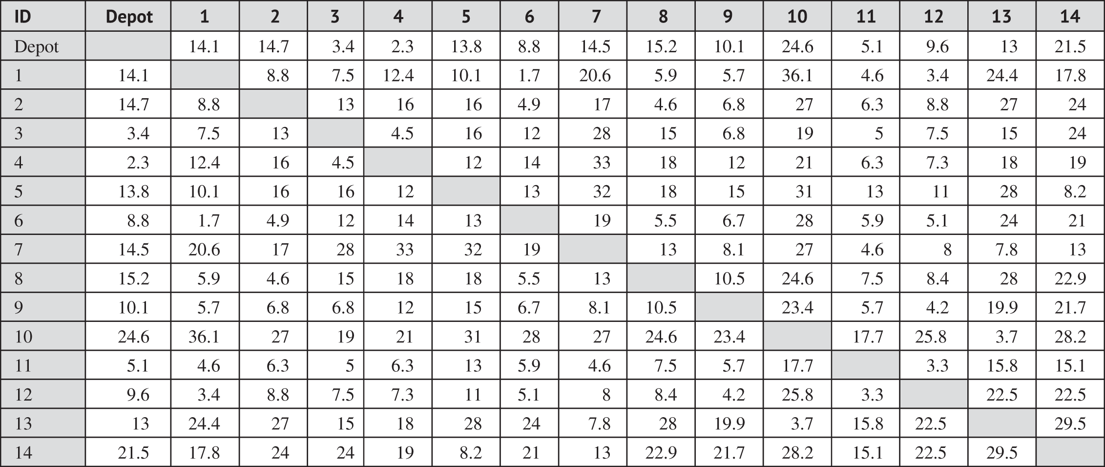
In Table 13.2, the driving distance between two consumers is presented in km. For this case, we recollected the driving distance in one direction and assume a symmetric matrix of distances. In addition, the distances were multiplied by a cost factor of 1.06$ by kilometer approximately to get the transport cost.
Table 13.2 Driving distance between locations of customers in kilometers.
 |
The delivery of the product was programmed over three periods and the maximum capacity in the truck was stated as 30 tons (just one vehicle).
13.4.1.1 The Inventory Routing Problem Under Certainty
The solution for this case was obtained in 231.7 seconds. Two routes were created for the periods first and second. In the third period, there weren't programmed deliveries.
- In the first period, the visit order of consumers was: Depot → C0 → C4 → C3 → C1 → C2 → C11 → Depot. The total product delivered with this route was 25.08 tons (83.6% of vehicle capacity).
- The second route was: Depot → C3 → C10 → C13 → C7 → C14 → C11 → Depot. And the total of products delivered is 27.9 (93% of vehicle capacity).
In the generated routes, the consumers C1, C2, C3, and C4 are first visited (health sector) and then the route can visit the costumers of the industry sector. The consumers C5, C6, C8, C9, and C12 are not visited along the periods, but for example, when six periods of planning are contemplated, the C5 and C9 are not programmed in route by their low rate of consumption. The total cost obtained was 330.34.
13.4.1.2 The Inventory Routing Problem Under Uncertainty in the Consumption Rate of Product
After assessing the uncertainty over the consumption rate of the product, a representation of the values through triangular fuzzy numbers was applied. To establish the left and right values for the triangular fuzzy number, the ± percentage of variation of 5%, 10%, and 15% over the original consumption rate was applied. The security degrees considered for this case for the given 4 values were 0, 0.50, 0.75, and 1, respectively.
To solve each case considering uncertainty in the consumption rate of the product, the constraints that involve these values were transformed in order to have a model with crisp values. The method applied was as defined by Adamo [28] as the righter value when a α− cut is defined under a degree of security.
In Table 13.3, the solution times and total cost are presented. The solution time in most cases was less than 5 minutes.
Table 13.3 Solution times and total costs.
| Variation (±%) | Security degree (α) | Solution time (seconds) | Total cost |
|---|---|---|---|
| 5 | 0 | 202.5 | 339.9 |
| 0.50 | 201.3 | 333.3 | |
| 0.75 | 165.1 | 332.1 | |
| 10 | 0 | 620.6 | 358.6 |
| 0.50 | 166.7 | 339.9 | |
| 0.75 | 195.0 | 333.3 | |
| 15 | 0 | 685.2 | 365.8 |
| 0.50 | 567.3 | 353.9 | |
| 0.75 | 244.8 | 334.6 | |
| 5, 10, 15 | 1 | 231.7 | 330.34 |
In the case when up to a percentage of decrement and increment occurs over the rate of consumption of a product, the total cost is impacted. When the percentage of variation is 5%, and the security degree is 0, the total cost is 339.9. Then with a 10% and a 15% of variation were 358.6 and 365.8, respectively. When the security degree increases, then the total cost reduces, then the total cost is reduced. Naturally, the highest cost is obtained when there is more variation and the security degree is the lowest (0) given that, a lower degree of security shows a lower level of knowledge. Also, the case when the highest cost was obtained (365.8) also implied the highest solution time (685.2).
13.5 Conclusions and Future Work
A mathematical model inspired by previous IRP formulations was developed incorporating priority in the deliveries for a certain group of customers. In the first experiment, we observed that the computational time of the solution increases very fast as well as the number of customers increases. However, one of the main objectives of this study was to show how the incorporation of uncertainty in demand besides the priority of customers in the health sector can be treated by the representation of fuzzy numbers and applying a defuzzification method.
In general, when the method of defuzzification is applied considering a α‐cut, with α as the security degree, the results show that the more α is reduced, the more the total cost (of inventory and transportation) increases. Naturally, the solution will be impacted by the grade of knowledge or the security degree that is established.
As future research, we are looking to develop new formulations that allow us to understand the behavior of the problem with the priority in deliveries as the new characteristic proposed in this chapter. Also, to make the problem closer to reality, it is important to incorporate other characteristics like vehicle fleet of different capacities, integrate IRP with the production planning problem, and consider aspects related to transport companies.
It is well known that IRP is a complex problem even with tens of customers and it will be required to develop non‐exact methods to solve bigger real instances in the future.
References
- 1 Herer, Y.T. and Levy, R. (1997). The metered inventory routing problem, an integrative heuristic algorithm. International Journal of Production Economics 51 (1): 69–81.
- 2 Campbell, A., Clarke, L., Kleywegt, A., and Savelsbergh, M. (1997). The Inventory Routing Problem in Fleet Management and Logistics (ed. C.T. Gabriel and L. Gilbert), 95–113. Spring US.
- 3 Moin, N.H. and Salhi, S. (2007). Inventory routing problems: a logistical overview. Journal of the Operational Research Society 58 (9): 1185–1194.
- 4 Yugang, Y., Haoxun, C., and Feng, C. (2008). A new model and hybrid approach for large scale inventory routing problems. European Journal of Operational Research 189 (3): 1022–1040.
- 5 Cordeau, J., Laport, G., Savelsbergh, M., and Vigo, D. (2007). Vehicle Routing in Handbooks in Operations Research and Management, edited by Barnhart Cynthia, Laporte Gilbert, 367‐428. Elsevier.
- 6 Archetti, C., Bianchessi, N., Irnich, S., and Speranza, M.G. (2014). Formulations for an inventory routing problem. International Transactions in Operational Research 21 (3): 353–374.
- 7 Andersson, H., Hoff, A., Christiansen, M., and Hasle, G. (2010). Industrial aspects and literature survey: Combined inventory management and routing. Computers & Operations Research 37 (9): 1515–1536.
- 8 Coelho, L.C., Cordeau, J., and Laporte, G. (2014). Thirty Years of Inventory Routing. Transportation Science 48 (1): 1–19.
- 9 Roldán, R.F., Basagoiti, R., and Coelho, L.C. (2017). A survey on the inventory‐routing problem with stochastic lead times and demands. Journal of Applied Logic 24 (1): 15–24.
- 10 Malladi, K.T. and Sowlati, T.S. (2018). Sustainability aspects in inventory routing problem: a review of new trends in the literature. Journal of Cleaner Production 197 (1): 804–814.
- 11 Savelsbergh, M. and Jin‐Hwa, S. (2007). Inventory routing with continuous moves. Computers & Operations Research 34 (6): 1744–1763.
- 12 Athanassios, N. and Ioannis, G. (2017). Economic model predictive inventory routing and control. Central European Journal of Operations Research 25 (3): 587–609.
- 13 Bard, J.F. and Nananukul, N. (2009). Heuristics for a multiperiod inventory routing problem with production decisions. Computers & Industrial Engineering 57 (3): 713–723.
- 14 Vansteenwegen, P. and Mateo, M. (2014). An iterated local search algorithm for the single‐vehicle cyclic inventory routing problem. European Journal of Operational Research 237 (3): 802–813.
- 15 Iassinovskaia, G., Limbourg, S., and Riane, F. (2017). The inventory‐routing problem of returnable transport items with time windows and simultaneous pickup and delivery in closed‐loop supply chains. International Journal of Production Economics 183 (1): 570–582.
- 16 Archetti, C., Christiansen, M., and Speranza, M.G. (2018). Inventory routing with pickups and deliveries. European Journal of Operational Research 268 (1): 314–324.
- 17 Naccache, S., Cordeau, J.F., and Coelho, L.C. (2018). The multi‐pickup and delivery problem with time windows. European Journal of Operational Research 269 (1): 353–362.
- 18 Moin, N.H., Salhi, S., and Aziz, N.A.B. (2011). An efficient hybrid genetic algorithm for the multi‐product multi‐period inventory routing problem. International Journal of Production Economics 133 (1): 334–343.
- 19 Coelho, L.C., Cordeau, J., and Laporte, G. (2012). Consistency in multi‐vehicle inventory‐routing. Transportation Research Part C: Emerging Technologies 24 (1): 270–287.
- 20 Solyali, O., Cordeau, J.F., and Laporte, G. (2014). Robust inventory routing under demand uncertainty. Transportation Science 46 (3): 327–340.
- 21 Bertazzi, L., Bosco, A., Guerriero, F., and Lagana, D. (2013). A stochastic inventory routing problem with stock‐out. Transportation Research Part C: Emerging Technologies 27 (1): 89–107.
- 22 Moin, N., Hasnah, H., and Huda, Z.A. (2018). Solving inventory routing problem with stochastic demand. AIP Conference Proceedings 1974 (1).
- 23 Niakan, F. and Rahimi, M. (2015). A multi‐objective healthcare inventory routing problem; a fuzzy possibilistic approach. Transportation Research Part E: Logistics and Transportation Review 80 (1): 74–94.
- 24 Qamsari, A., Saeed, N., Motlagh, S. et al. (2020). A column generation approach for an inventory routing problem with fuzzy time windows. Operational Research.
- 25 Micheli Guido, J.L. and Mantella, F. (2018). Modelling an environmentally‐extended inventory routing problem with demand uncertainty and a heterogeneous fleet under carbon control policies. International Journal of Production Economics 204: 316–327.
- 26 Avila‐Torres, P., Caballero, R., Litvinchev, I. et al. (2018). The urban transport planning with uncertainty in demand and travel time: a comparison of two defuzzification methods. Journal of Ambient Intelligence and Humanized Computing 9 (3): 843–856.
- 27 Campos, L. and Verdegay, J.L. (1989). Linear programming problems and ranking of fuzzy numbers. Fuzzy Sets and Systems 32 (1): 1–11.
- 28 Adamo, J.M. (1980). Fuzzy decision trees. Fuzzy Sets and Systems 4: 207–219.
- 29 Brunelli, M. and Mezei, J. (2013). How different are ranking methods for fuzzy number? A numerical study. Internal Journal of Approximate Reasoning 54: 627–639.
- 30 Archetti, C., Bertazzi, L., Laporte, G., and Speranza, M.G. (2007). A branch‐and‐cut algorithm for a vendor‐managed inventory‐routing problem. Transportation Science 41 (3): 382–391.