© Abhishek Singh, Karthik Ramasubramanian, Shrey Shivam  2019
A. Singh et al.Building an Enterprise Chatbothttps://doi.org/10.1007/978-1-4842-5034-1_5

5. Natural Language Processing, Understanding, and Generation

Abhishek Singh1 , Karthik Ramasubramanian1 and Shrey Shivam2
(1)
New Delhi, Delhi, India
(2)
Donegal, Donegal, Ireland
 

The human brain is one of the most advanced machines when it comes to processing, understanding, and generating (P-U-G) natural language. The capabilities of the human brain stretch far beyond just being able to perform P-U-G on one language, dialect, accent, and conversational undertone. No machine has so far reached the human potential of performing all three tasks seamlessly. However, the advances in machine learning algorithms and computing power are making the distant dream of creating human-like bots a possibility.

In this chapter, we will explore the P-U-G of natural languages and their nuances with references to use cases and examples. Table 5-1 provides a quick summary of natural language processing (NLP), natural language understanding (NLU), and natural language generation (NLG) with a few functions and real-world applications. We will get into more details on natural language processing, understanding, and generation in their respective sections.
Table 5-1

NLP, NLU, and NLG

Type

NLP

NLU

NLG

Brief

Process and analyze written or spoken text by breaking it down, comprehending its meaning, and determining the appropriate action. It involves parsing, sentence breaking, and stemming.

A specific type of NLP that helps to deal with reading comprehension, which includes the ability to understand meaning from its discourse content and identify the main thought of a passage.

NLG is one of the tasks of NLP to generate natural language text from structured data from a knowledge base. In other words, it transforms data into a written narrative.

Functions

Identify part of speech, text categorizing, named entity recognition, translation, speech recognition

Automatic summarization, semantic parsing, question answering, sentiment analysis

Content determination, document structuring, generating text in interactive conversation

Real-World Application

Article classification for digital news aggregation company

Building a Q&A chatbot, brand sentiment using Twitter and Facebook data

Generating a product description for an e-commerce website or a financial portfolio summary

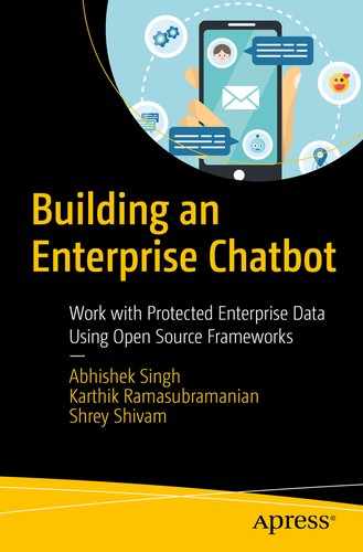
Chatbot Architecture

When it comes to building an enterprise chatbot, you have so far seen how to identify data sources, design the chatbot architecture, list business use cases, and many other concepts that help an enterprise to process efficiently, reduce manual labor, and reduce the cost of operations. In this chapter, we will focus on the core part of a chatbot: the ability to process textual data and take part in a human-like conversation. Figure 5-1 shows an architecture that utilizes the techniques from NLP, NLU, and NLG to build an enterprise chatbot.
../images/478492_1_En_5_Chapter/478492_1_En_5_Fig1_HTML.jpg
Figure 5-1

Architecture diagram for chatbots

Let’s say an airline company has built a chatbot to book a flight via their website or social media pages. The following are the steps as per the architecture shown in Figure 5-1:
  1. 1.

    Customer says, “Help me book a flight for tomorrow from London to New York” through the airline’s Facebook page. In this case, Facebook becomes the presentation layer. A fully functional chatbot could be integrated into a company’s website, social network page, and messaging apps like Skype and Slack.

     
  2. 2.

    Next, the message is carried to the messaging backend where the plain text passes through an NLP/NLU engine, where the text is broken into tokens, and the message is converted into a machine-understandable command. We will revisit this in greater detail throughout this chapter.

     
  3. 3.

    The decision engine then matches the command with preconfigured workflows. So, for example, to book a flight, the system needs a source and a destination. This is where NLG helps. The chatbot will ask, “Sure, I will help in you booking your flight from London to New York. Could you please let me know if you prefer your flight from Heathrow or Gatwick Airport?” The chatbot picks up the source and destination and automatically generates a follow-up question asking which airport the customer prefers.

     
  4. 4.

    The chatbot now hits the data layer and fetches the flight information from prefed data sources, which could typically be connected to live booking systems. The data source provides flight availability, price, and many other services as per the design.


Some chatbots are heavy on generative responses, and others are built for retrieving information and fitting it in a predesigned conversational flow. For example, in the flight booking use case, we almost know all the possible ways the customer could ask to book a flight, whereas if we take an example of a chatbot for a telemedicine company, we are not sure about all the possible questions a patient could ask. So, in the telemedicine company chatbot, we need the help of generative models built using NLG techniques, whereas in the flight booking chatbot, a good retrieval-based system with NLP and an NLP engine should work.

Since this book is about building an enterprise chatbot, we will focus more on the applications of P-U-G in natural languages rather than going deep into the foundations of the subject. In the next section, we’ll show various techniques for NLP and NLU using some of the most popular tools in Python. There are other Java and C# bases libraries; however, Python libraries provide more significant community support and faster development.

Further, to differentiate between NLP and NLU, the Venn diagram in Figure 5-2 shows a few applications of NLP and NLU. It shows NLU as a subset of NLP. The segregation is only in the tasks, not in the scope. The overall objective is to process and understand the natural language text to make machines think like humans.
../images/478492_1_En_5_Chapter/478492_1_En_5_Fig2_HTML.jpg
Figure 5-2

Applications of NLP and NLU

Popular Open Source NLP and NLU Tools

In this section, we will briefly explore various open source tools available to perform natural language processing, understanding, and generation. While each of these tools does not differentiate between the P-U-G of natural language, we will demonstrate the capabilities of tools under the corresponding three separate headings.

NLTK

The Natural Language Toolkit (NLTK) is a Python library for processing English vocabulary. It has an Apache 2.0 open source license. NLTK is written in the Python programming language. The following are some of the tasks NLTK can perform:
  • Classification of text: Classifying text into a different category for better organization and content filtering

  • Tokenization of sentences: Breaking sentences into words for symbolic and statistical natural language processing

  • Stemming words: Reducing words into base or root form

  • Part-of-speech (POS) tagging: Tagging the words into POS, which categorizes the words into similar grammatical properties

  • Parsing text: Determining the syntactic structure of text based on the underlying grammar

  • Semantic reasoning: Ability to understand the meaning of the word to create representations

NLTK is the first choice of a tool for teaching NLP. It is also widely used as a platform for prototyping and research.

spaCy

Most organizations that build a product involving natural language data are adapting spaCy. It stands out with its offering of a production-grade NLP engine that is accurate and fast. With the extensive documentation, the adaption rate further increases. It is developed in Python and Cython. All the language models in spaCy are trained using deep learning, which provides high accuracy for all NLP tasks.

Currently, the following are some high-level capabilities of spaCy:
  • Covers NLTK features: Provides all the features of NLTK-like tokenization, POS tagging, dependency trees, named entity recognition, and many more.

  • Deep learning workflow: spaCy supports deep learning workflows, which can connect to models trained on popular frameworks like Tensorflow, Keras, Scikit-learn, and PyTorch. This makes spaCy the most potent library when it comes to building and deploying sophisticated language models for real-world applications.

  • Multi-language support: Provides support for more than 50 languages including French, Spanish, and Greek.

  • Processing pipeline: Offers an easy-to-use and very intuitive processing pipeline for performing a series of NLP tasks in an organized manner. For example, a pipeline for performing POS tagging, parsing the sentence, and named the entity extraction could be defined in a list like this: pipeline = ["tagger," "parse," "ner"]. This makes the code easy to read and quick to debug.

  • Visualizers: Using displaCy, it becomes easy to draw a dependency tree and entity recognizer. We can add our colors to make the visualization aesthetically pleasing and beautiful. It quickly renders in a Jupyter notebook as well.

CoreNLP

Stanford CoreNLP is one of the oldest and most robust tools for all natural language tasks. Its suite of functions offers many linguistic analysis capabilities, including the already discussed POS tagging, dependency tree, named entity recognition, sentiment analysis, and others. Unlike spaCy and NLTK, CoreNLP is written in Java. It also provides Java APIs to use from the command line and third-party APIs for working with modern programming languages. The following are the core features of using CoreNLP:
  • Fast and robust: Since it is written in Java, which is a time-tested and robust programming language, CoreNLP is a favorite for many developers.

  • A broad range of grammatical analysis: Like NLTK and spaCy, CoreNLP also provides a good number of analytical capabilities to process and understand natural language.

  • API integration: CoreNLP has excellent API support for running it from the command line and programming languages like Python via a third-party API or web service.

  • Support multiple Operating Systems (OSs): CoreNLP works in Windows, Linux, and MacOS.

  • Language support: Like spaCy, CoreNLP provides useful language support, which includes Arabic, Chinese, and many more.

gensim

gensim is a popular library written in Python and Cython. It is robust and production-ready, which makes it another popular choice for NLP and NLU. It can help analyze the semantic structure of plain-text documents and come out with important topics. The following are some core features of gensim:
  • Topic modeling: It automatically extracts semantic topics from documents. It provides various statistical models, including latent Dirichlet analysis (LDA) for topic modeling.

  • Pretrained models: It has many pretrained models that provide out-of-the-box capabilities to develop general-purpose functionalities quickly.

  • Similarity retrieval: gensim’s capability to extract semantic structures from any document makes it an ideal library for similarity queries on numerous topics.

Table 5-2 from the spaCy website summarizes if a given NLP feature is available in NLTK, spaCy, and CoreNLP.
Table 5-2

Features available in spaCy, NLTK, and CoreNLP

S.No.

Feature

spaCy

NLTK

CoreNLP

1

Programming language

Python

Python

Java/Python

2

Neural network models

Yes

No

Yes

3

Integrated word vectors

Yes

No

No

4

Multi-language support

Yes

Yes

Yes

5

Tokenization

Yes

Yes

Yes

6

Part-of-speech tagging

Yes

Yes

Yes

7

Sentence segmentation

Yes

Yes

Yes

8

Dependency parsing

Yes

No

Yes

9

Entity recognition

Yes

Yes

Yes

10

Entity linking

No

No

No

11

Coreference resolution

No

No

Yes

TextBlob

TextBlob is a relatively less popular but easy-to-use Python library that provides various NLP capabilities like the libraries discussed above. It extends the features provided by NLTK but in a much-simplified form. The following are some of the features of TextBlob:
  • Sentiment analysis: It provides an easy-to-use method for computing polarity and subjectivity kinds of scores that measures the sentiment of a given text.

  • Language translations: Its language translation is powered by Google Translate, which provides support for more than 100 languages.

  • Spelling corrections: It uses a simple spelling correction method demonstrated by Peter Norvig on his blog at http://norvig.com/spell-correct.html . Currently the Engineering Director at Google, his approach is 70% accurate.

fastText

fasText is a specialized library for learning word embeddings and text classification. It was developed by researchers in Facebook’s FAI Research (FAIR) lab. It is written in C++ and Python, making it very efficient and fast in processing even a large chunk of data. The following are some of the features of fastText:
  • Word embedding learnings: Provides many word embedding models using skipgram and Continous Bag of Words (CBOW) by unsupervised training.

  • Word vectors for out-of-vocabulary words: It provides the capability to obtain word vectors even if the word is not present in the training vocabulary.

  • Text classification: fastText provides a fast text classifier, which in their paper titled “Bag of Tricks for Efficient Text Classification” claims to be often at par with many deep learning classifiers’ accuracy and training time.

In the next few sections, you will see how to apply these tools to perform various tasks in NLP, NLU, and NLG.

Natural Language Processing

Language skills are considered the most sophisticated tasks that a human can perform. Natural language processing deals with understanding and manicuring natural language text or speech to perform specific useful desired tasks. NLP combines ideas and concepts from computer science, linguistics, mathematics, artificial intelligence, machine learning, and psychology.

Mining information from unstructured textual data is not as straightforward as performing a database query using SQL. Categorizing documents based on keywords, identifying a mention of a brand in a social media post, and tracking the popularity of a leader on Twitter are all possible if we can identify entities like a person, organization, and other useful information.

The primary tasks in NLP are processing and analyzing written or spoken text by breaking it down, comprehending its meaning, and determining appropriate action. It involves parsing, sentence breaking, stemming, dependency tree, entity extraction, and text categorization.

We will see how words in a language are broken into smaller tokens and how various transformations work (transforming textual data into a structured and numeric value). We will also explore popular libraries like NLTK, TextBlob, spaCy, CoreNLP, and fastText.

Processing Textual Data

We will use the Amazon Fine Food Review dataset throughout this chapter for all demonstrations using various open-source tools. The dataset can be downloaded from www.kaggle.com/snap/amazon-fine-food-reviews , which is made available with a CC0: Public Domain license.

Reading the CSV File

Using a read_csv function from the pandas library, we read the Reviews.csv file into a food_review data frame and print the top rows (Figure 5-3):
import pandas as pd
food_review = pd.read_csv("Reviews.csv")
food_review.head()
../images/478492_1_En_5_Chapter/478492_1_En_5_Fig3_HTML.jpg
Figure 5-3

A CSV file

As can be seen, the CSV contains columns like ProductID, UserID, Product Rating, Time, Summary, and Text of the review. The file contains almost 500K reviews for various products. Let’s sample some reviews to process.

Sampling

Using the sample function from the pandas data frame, let’s randomly pick the text of 1000 reviews and print the top rows (see Figure 5-4):
food_review_text = pd.DataFrame(food_review["Text"])
food_review_text_1k = food_review_text.sample(n= 1000,random_state = 123)
food_review_text_1k.head()
../images/478492_1_En_5_Chapter/478492_1_En_5_Fig4_HTML.jpg
Figure 5-4

Samples

Tokenization Using NLTK

As discussed, NLTK offers many features for processing textual data. The first step in processing text data is to separate a sentence into individual words. This process is called tokenization. We will use the NLTK’s word_tokenize function to create a column in the food_review_text_1k data frame we created above and print the top six rows to see the output of tokenize (Figure 5-5):
food_review_text_1k['tokenized_reviews'] = food_review_text_1k['Text'].apply(nltk.word_tokenize)
food_review_text_1k.head()
../images/478492_1_En_5_Chapter/478492_1_En_5_Fig5_HTML.jpg
Figure 5-5

Top rows

Word Search Using Regex

Now that we have the tokenized text for each review, let’s take the first row in the data frame and search for the presence of the word using a regular expression (regex) . The regex searches for any word that contains c as its first character and i as the third character. We can write various regex searches for a pattern of interest. We use the re.search() function to perform this search:
#Search: All 5-letter words with c as its first letter and i as its third letter
search_word = set([w for w in food_review_text_1k['tokenized_reviews'].iloc[0] if re.search('^c.i..$', w)])
print(search_word)
{'chips'}

Word Search Using the Exact Word

Another way of searching for a word is to use the exact word. This can be achieved using the str.contains() function in pandas. In the following example, we search for the word “great” in all of the reviews. The rows of the reviews containing the word will be retrieved. They can be considered a positive review. See Figure 5-6.
#Search for the word "great" in reviews
food_review_text_1k[food_review_text_1k['Text'].str.contains('great')]
../images/478492_1_En_5_Chapter/478492_1_En_5_Fig6_HTML.jpg
Figure 5-6

Samples with a specific word

NLTK

In this section, we will use many of the features from NLTK for NLP, such as normalization, noun phrase chunking, named entity recognition, and document classifier.

Normalization Using NLTK

In many natural language tasks, we often deal with the root form of the words. For example, for the words “baking” and “baked,” the root word is “bake.” This process of extracting the root word is called stemming or normalization. NLTK provides two functions implementing the stemming algorithm. The first is the Porter Stemming algorithm, and the second is the Lancaster stemmer.

There are slight differences in the quality of output from both algorithms. For example, in the following example, the Porter stemmer converts the word “sustenance” into “sustain” while the Lancaster stemmer outputs “sust.”
words = set(food_review_text_1k['tokenized_reviews'].iloc[0])
print(words)
porter = nltk.PorterStemmer()
print([porter.stem(w) for w in words])
Before
{'when', 'always', 'great', 'vending', 'for', 'make', "'m", 'just', 'I', '.', 'love', 'a', 'They', 'with', 'healthy', 'these', 'snack', 'the', 'at', 'work', 'chips', 'machine', 'stuck', 'sustenance', '!'}
After
['when', 'alway', 'great', 'vend', 'for', 'make', "'m", 'just', 'I', '.', 'love', 'a', 'they', 'with', 'healthi', 'these', 'snack', 'the', 'at', 'work', 'chip', 'machin', 'stuck', 'susten', '!']
lancaster = nltk.LancasterStemmer()
print([lancaster.stem(w) for w in words])
['when', 'alway', 'gre', 'vend', 'for', 'mak', "'m", 'just', 'i', '.', 'lov', 'a', 'they', 'with', 'healthy', 'thes', 'snack', 'the', 'at', 'work', 'chip', 'machin', 'stuck', 'sust', '!']

Noun Phrase Chunking Using Regular Expressions

Above you saw the tokens as a fundamental unit in any NLP processing. Since in natural language, a group of tokens combined often reveals the meaning or represents a concept, we create chunks. Multi-token sequences are created by segmenting using a process called chunking. In Figure 5-7, the smaller boxes show word-level tokenization and the larger boxes shows multi-token sequences, also called higher-level chunks. Such chunks are created using regular expressions or by using the n-gram (more on this in later sections) method. Chunking is essential for entity recognition, which we will shortly explore.
../images/478492_1_En_5_Chapter/478492_1_En_5_Fig7_HTML.jpg
Figure 5-7

Tokens and chunks

Let’s consider a single review as shown in the following code. The grammar finds a noun using a rule that says, find noun chunk where zero or one (?) determiner (DT) is followed by any number (*) of adjectives (JJ) and a noun (NN). In the POS tree shown in the output of the following code, all the chunks marked as NP are the noun phrases:
import nltk
from nltk.tokenize import word_tokenize
#Noun phrase chunking
text = word_tokenize("My English Bulldog Larry had skin allergies the summer we got him at age 3, I'm so glad that now I can buy his food from Amazon")
#This grammar rule: Find NP chunk when an optional determiner (DT) is followed by any number of adjectives (JJ) and then a noun (NN)
grammar = "NP: {<DT>?<JJ>*<NN>}"
#Regular expression parser using the above grammar
cp = nltk.RegexpParser(grammar)
#Parsed text with pos tag
review_chunking_out = cp.parse(nltk.pos_tag(text))
#Print the parsed text
print(review_chunking_out)
(S
  My/PRP$
  English/JJ
  Bulldog/NNP
  Larry/NNP
  had/VBD
  skin/VBN
  allergies/NNS
  (NP the/DT summer/NN)
  we/PRP
  got/VBD
  him/PRP
  at/IN
  (NP age/NN)
  3/CD
  ,/,
  I/PRP
  'm/VBP
  so/RB
  glad/JJ
  that/IN
  now/RB
  I/PRP
  can/MD
  buy/VB
  his/PRP$
  (NP food/NN)
  from/IN
  Amazon/NNP)
You can see many NPs such as “the summer” and “age” where “the summer” is not a single word token. Above you see that the POS is in a tree representation. Another way of representing the chunk structures is by using tags. The IOB tag representation is a general standard. In this scheme, each token is represented as I (Inside), O (Outside), and B (Begin). Chunk tag B represents the beginning of a chunk. Subsequent tokens within a chunk are tagged I and all other tokens are tagged O. Figure 5-8 provides one example of an IOB tag representation.
../images/478492_1_En_5_Chapter/478492_1_En_5_Fig8_HTML.jpg
Figure 5-8

IOB tag representation of chunk structures

The following code uses the CoNLL 2000 Corpus to convert the tree to tags using the function tree2conlltags(). CoNLL is Wall Street Journal text that has been tagged and chunked using IOB notation.
from nltk.chunk import conlltags2tree, tree2conlltags
from pprint import pprint
#Print IOB tags
review_chunking_out_IOB = tree2conlltags(review_chunking_out)
pprint(review_chunking_out_IOB)
[('My', 'PRP$', 'O'),
 ('English', 'JJ', 'O'),
 ('Bulldog', 'NNP', 'O'),
 ('Larry', 'NNP', 'O'),
 ('had', 'VBD', 'O'),
 ('skin', 'VBN', 'O'),
 ('allergies', 'NNS', 'O'),
 ('the', 'DT', 'B-NP'),
 ('summer', 'NN', 'I-NP'),
 ('we', 'PRP', 'O'),
 ('got', 'VBD', 'O'),
 ('him', 'PRP', 'O'),
 ('at', 'IN', 'O'),
 ('age', 'NN', 'B-NP'),
 ('3', 'CD', 'O'),
 (',', ',', 'O'),
 ('I', 'PRP', 'O'),
 ("'m", 'VBP', 'O'),
 ('so', 'RB', 'O'),
 ('glad', 'JJ', 'O'),
 ('that', 'IN', 'O'),
 ('now', 'RB', 'O'),
 ('I', 'PRP', 'O'),
 ('can', 'MD', 'O'),
 ('buy', 'VB', 'O'),
 ('his', 'PRP$', 'O'),
 ('food', 'NN', 'B-NP'),
 ('from', 'IN', 'O'),
 ('Amazon', 'NNP', 'O')]

Named Entity Recognition

Once we have the POS of the text, we can extract the named entities. Named entities are definite noun phrases that refer to specific individuals such as ORGANIZATION and PERSON. Some other entities are LOCATION, DATE, TIME, MONEY, PERCENT, FACILITY, and GPE. The facility is any human-made artifact in the architecture and civil engineering domain, such as Taj Mahal or Empire State Building. GPE means geopolitical entities such as city, state, and country. We can extract all these entities using the ne_chunk() method in the nltk library.

The following code uses the POS tagged sentence and applies the ne_chunk() method to it. It identifies Amazon as GPE and Bulldog Larry as a PERSON. In this case, this is both true and false. Amazon is identified as ORGANIZATION, which we expect here. Later in the chapter, we will train our own named entity recognizer to improve the performance.
tagged_review_sent = nltk.pos_tag(text)
print(nltk.ne_chunk(tagged_review_sent))
(S
  My/PRP$
  English/JJ
  (PERSON Bulldog/NNP Larry/NNP)
  had/VBD
  skin/VBN
  allergies/NNS
  the/DT
  summer/NN
  we/PRP
  got/VBD
  him/PRP
  at/IN
  age/NN
  3/CD
  ,/,
  I/PRP
  'm/VBP
  so/RB
  glad/JJ
  that/IN
  now/RB
  I/PRP
  can/MD
  buy/VB
  his/PRP$
  food/NN
  from/IN
  (GPE Amazon/NNP))

spaCy

While spaCy offers all the features of NLTK, it is regarded as one of the best production grade tools for an NLP task. In this section, we will see how to use the various methods provided by the spaCy library in Python.

spaCy provides three core models: en_core_web_sm (10MB), en_core_web_md (91MB), and en_core_web_lg (788MB). The larger model is trained on bigger vocabulary and hence will give higher accuracy. So depending on your use case, choose wisely the model that fits your requirements.

POS Tagging

After loading the model using spaCy.load(), you can pass any string to the model, and it provides all the methods in one go. To extract POS, the pos_method is used. In the following code, after tokenizing, we print the following:
  • text: The original text

  • lemma: Token after stemming, which is the base form of the word

  • pos: Part of speech

  • tag: POS with details

  • dep: The relationship between the tokens. Also called syntactical dependency.

  • shape: The shape of the word (i.e., capitalization, punctuation, digits)

  • is_alpha: Returns True if the token is an alphanumeric character

  • is.stop: Returns True if the token is a stopword like “at,” “so,” etc.

# POS tagging
import spacy
nlp = spacy.load('en_core_web_sm')
doc = nlp(u"My English Bulldog Larry had skin allergies the summer we got him at age 3, I'm so glad that now I can buy his food from Amazon")
for token in doc:
    print(token.text, token.lemma_, token.pos_, token.tag_, token.dep_, token.shape_, token.is_alpha, token.is_stop)
My -PRON- DET PRP$ poss Xx True True
English English PROPN NNP compound Xxxxx True False
Bulldog Bulldog PROPN NNP nsubj Xxxxx True False
Larry Larry PROPN NNP nsubj Xxxxx True False
had have VERB VBD ccomp xxx True True
skin skin NOUN NN compound xxxx True False
allergies allergy NOUN NNS dobj xxxx True False
the the DET DT det xxx True True
summer summer NOUN NN npadvmod xxxx True False
we -PRON- PRON PRP nsubj xx True True
got get VERB VBD relcl xxx True False
him -PRON- PRON PRP dobj xxx True True
at at ADP IN prep xx True True
age age NOUN NN pobj xxx True False
3 3 NUM CD nummod d False False
, , PUNCT, punct, False False
I -PRON- PRON PRP nsubj X True True
'm be VERB VBP ROOT 'x False True
so so ADV RB advmod xx True True
glad glad ADJ JJ acomp xxxx True False
that that ADP IN mark xxxx True True
now now ADV RB advmod xxx True True
I -PRON- PRON PRP nsubj X True True
can can VERB MD aux xxx True True
buy buy VERB VB ccomp xxx True False
his -PRON- DET PRP$ poss xxx True True
food food NOUN NN dobj xxxx True False
from from ADP IN prep xxxx True True
Amazon Amazon PROPN NNP pobj Xxxxx True False

Dependency Parsing

The spaCy dependency parser has a rich API which helps to navigate the dependency tree. It also provides the capability to detect sentence boundaries and iterate through the noun phrase or chunks. In the following example, the noun_chunks method in the model is iteratable with the following methods:
  • text: Original noun chunk

  • root.text: Original word connecting the noun chunk to the rest of the noun chunk parse

  • root.dep: Dependency relation connecting the root to its head

  • root.head: Root token’s head

From the example, “My English Bulldog” is a noun phrase, where “Bulldog” is root text with “nsubj” relation and “had” as its root head.
#Dependency parse
import spacy
nlp = spacy.load("en_core_web_sm")
doc = nlp(u"My English Bulldog Larry had skin allergies the summer we got him at age 3, I'm so glad that now I can buy his food from Amazon")
for chunk in doc.noun_chunks:
    print(chunk.text, chunk.root.text, chunk.root.dep_,
            chunk.root.head.text)
My English Bulldog Bulldog nsubj had
Larry Larry nsubj had
skin allergies allergies dobj had
we we nsubj got
him him dobj got
age age pobj at
I I nsubj 'm
I I nsubj buy
his food food dobj buy
Amazon Amazon pobj from

Dependency Tree

spaCy provides a method called displayCy for visualization. We can draw the dependency tree of a given sentence using displaCy (see Figures 5-9, 5-10, and 5-11).
import spacy
from spacy import displacy
nlp = spacy.load("en_core_web_sm")
doc = nlp(u"My English Bulldog Larry had skin allergies the summer we got him at age 3")
displacy.render(doc, style="dep")
../images/478492_1_En_5_Chapter/478492_1_En_5_Fig9_HTML.jpg
Figure 5-9

Dependency tree, part 1

../images/478492_1_En_5_Chapter/478492_1_En_5_Fig10_HTML.jpg
Figure 5-10

Dependency tree, part 2

../images/478492_1_En_5_Chapter/478492_1_En_5_Fig11_HTML.jpg
Figure 5-11

Dependency tree, part 3

From the dependency trees, you can see that there are two compound word pairs, “English Bulldog” and “skin allergies,” and NUM “3” is the modifier of “age.” You can also see “summer” as the noun phrase as an adverbial modifier (npadvmod) to the token “had.” You can also observe many direct objects (dobj) of a verb phrase, which is a noun phrase, like (got, him) and (had, allergies) and object of a preposition (pobj) like (at, age). A detailed explanation of the relationships in a dependency tree can be found here: https://nlp.stanford.edu/software/dependencies_manual.pdf .

Chunking

spaCy provides an easy-to-use retrieval of chunk information such as VERB and NOUN from a given text. The noun_chunks method provides noun phrases, and from pos, we can search for VERB. The following code extracts noun phrases and verbs from the chunks:
# pip install spacy
# python -m spacy download en_core_web_sm
import spacy
# Load English tokenizer, tagger, parser, NER, and word vectors
nlp = spacy.load("en_core_web_sm")
# Process whole documents
text = ("My English Bulldog Larry had skin allergies the summer we got him at age 3, I'm so glad that now I can buy his food from Amazon")
doc = nlp(text)
# Analyze syntax
print("Noun phrases:", [chunk.text for chunk in doc.noun_chunks])
print("Verbs:", [token.lemma_ for token in doc if token.pos_ == "VERB"])
Noun phrases: ['My English Bulldog', 'Larry', 'skin allergies', 'we', 'him', 'age', 'I', 'I', 'his food', 'Amazon']
Verbs: ['have', 'get', 'be', 'can', 'buy']

Named Entity Recognition

spaCy has an accuracy of 85.85% in named entity recognition (NER) tasks. The en_core_web_sm model provides the function ents, which provides the entities. The model is trained on the OntoNotes dataset, which can be found at https://catalog.ldc.upenn.edu/LDC2013T19 .

The default models in spaCy provide the entities shown in Table 5-3.
Table 5-3

Types

TYPE

DESCRIPTION

PERSON

Names of people including fictional characters

NORP

Nationalities or religious or political groups

FAC

Civil engineering structures or infrastructures like buildings, airports, highways, bridges, etc.

ORG

Organization names like companies, agencies, institutions, etc.

GPE

A geopolitical entity like countries, cities, states

LOC

Non-GPE locations like mountain ranges, water bodies

PRODUCT

Objects, vehicles, foods, etc. (not services)

EVENT

Named hurricanes, battles, wars, sports events, etc.

WORK_OF_ART

Titles of books, songs, etc.

LAW

Named documents made into laws

LANGUAGE

Any named language

DATE

Absolute or relative dates or periods

TIME

Times smaller than a day

PERCENT

Percentage, including %

MONEY

Monetary values, including unit

QUANTITY

Measurements, as of weight or distance

ORDINAL

“first,” “second,” etc.

CARDINAL

Numerals that do not fall under another type

The following code extracts the English Bulldog Larry as a PERSON entity and Amazon as entity ORG. Unlike NLTK, where it identified Amazon as GPE, spaCy correctly identifies the context of the sentence to figure out that Amazon is an organization in the given sentence.
import spacy
# Load English tokenizer, tagger, parser, NER, and word vectors
nlp = spacy.load("en_core_web_sm")
# Process whole documents
text = ("My English Bulldog Larry had skin allergies the summer we got him at age 3, I'm so glad that now I can buy his food from Amazon")
doc = nlp(text)
# Find named entities
for entity in doc.ents:
    print(entity.text, entity.label_)
English Bulldog Larry PERSON
Amazon ORG
We can also visualize the entities using the displacy method (shown in Figure 5-12):
import spacy
from spacy import displacy
from pathlib import Path
text = "I found these crisps at our local WalMart & figured I would give them a try. They were so yummy I may never go back to regular chips, not that I was a big chip fan anyway. The only problem is I can eat the entire bag in one sitting. I give these crisps a big thumbs up!"
nlp = spacy.load("en_core_web_sm")
doc = nlp(text)
svg = displacy.serve(doc, style="ent")
output_path = Path("images/sentence_ne.svg")
output_path.open("w", encoding="utf-8").write(svg)
../images/478492_1_En_5_Chapter/478492_1_En_5_Fig12_HTML.jpg
Figure 5-12

Results

Pattern-Based Search

spaCy also provides a pattern or rule-based search. We can define our pattern on top of a function like LOWER. For example, in the following code, we define a search span as “Walmart” in lowercase followed by a punctuation mark. This pattern could be written like
pattern = [{"LOWER": "walmart"}, {"IS_PUNCT": True}]

In the search span, if we want to find the word “Walmart,” we define this using the matcher.add method and pass pattern as the argument to the method.

This syntax is more user-friendly than a cumbersome regular expression, which is hard to understand. The result of the search reveals that the word “Walmart” is found at the seventh position in the string and ends at the ninth position. The output also shows the span text as “Walmart &,” which we defined in the pattern.
# Spacy - Rule-based matching
import spacy
from spacy.matcher import Matcher
nlp = spacy.load("en_core_web_sm")
matcher = Matcher(nlp.vocab)
#Search for Walmart after converting the text in lower case and
pattern = [{"LOWER": "walmart"}, {"IS_PUNCT": True}]
matcher.add("Walmart", None, pattern)
doc = nlp(u"I found these crisps at our local WalMart & figured I would give them a try. They were so yummy I may never go back to regular chips, not that I was a big chip fan anyway. The only problem is I can eat the entire bag in one sitting. I give these crisps a big thumbs up!")
matches = matcher(doc)
for match_id, start, end in matches:
    string_id = nlp.vocab.strings[match_id]  # Get string representation
    span = doc[start:end]  # The matched span
    print(match_id, string_id, start, end, span.text)
16399848736434528297 Walmart 7 9 WalMart &

Searching for Entity

Using the matcher method, we can also search for a type of entity in a given text. In the following code, we search for the entity ORG (defined by “label”) named “walmart.”
from spacy.lang.en import English
from spacy.pipeline import EntityRuler
nlp = English()
ruler = EntityRuler(nlp)
patterns = [{"label": "ORG","pattern":[{"lower":"walmart"}]}]
ruler.add_patterns(patterns)
nlp.add_pipe(ruler)
doc = nlp(u"I found these crisps at our local WalMart & figured I would give them a try. They were so yummy I may never go back to regular chips, not that I was a big chip fan anyway. The only problem is I can eat the entire bag in one sitting. I give these crisps a big thumbs up!")
print([(ent.text, ent.label_) for ent in doc.ents])
[('WalMart', 'ORG')]

Training a Custom NLP Model

In many real-world datasets, the entities are not detected as per the expectations. The models in spaCy or NLTK are not trained on those words or tokens. In such cases, we can train a custom model using a private dataset. We have to create training data in a particular format. In the following code, we pick two sentences and tag an entity PRODUCT with its start and end position in the text. The syntax looks like this:
(
    u"As soon as I tasted one and it tasted like a corn chip I checked the ingredients. ",
    {
    "entities": [(45, 49, "PRODUCT")]
    }
)
We tag the food product “corn” in the two sentences. Here we take just two sentences, and spaCy trains the model well with just them. If you don’t get the right entity with a smaller dataset, you might need to add a few more examples before the model will pick the right entity.
import spacy
import random
train_data = [
        (u"As soon as I tasted one and it tasted like a corn chip I checked the ingredients. ", {"entities": [(45, 49, "PRODUCT")]}),
        (u"I found these crisps at our local WalMart & figured I would give them a try", {"entities": [(14, 20, "PRODUCT")]})
]
other_pipes = [pipe for pipe in nlp.pipe_names if pipe != "ner"]
with nlp.disable_pipes(*other_pipes):
    optimizer = nlp.begin_training()
    for i in range(10):
        random.shuffle(train_data)
        for text, annotations in train_data:
            nlp.update([text], [annotations], sgd=optimizer)
nlp.to_disk("model/food_model")
We saved the trained model to disk and named it food_model. In the following code, we load the food_model from disk and try to predict the entity on a test sentence. We see it does a good job here in identifying corn as a PRODUCT entity.
import spacy
nlp = spacy.load("model/food_model")
text = nlp("I consume about a jar every two weeks of this, either adding it to fajitas or using it as a corn chip dip")
for entity in text.ents:
    print(entity.text, entity.label_)
corn PRODUCT

CoreNLP

CoreNLP is another popular toolkit for linguistic analysis such as POS tagging, dependency tree, named entity recognition, sentiment analysis, and many others. We are going to use the CoreNLP features from Python through a third-party wrapper called Stanford-corenlp. It can be installed using pip install in the command line or cloned from GitHub here: https://github.com/Lynten/stanford-corenlp .

Once you install or download the code, you need to specify the path to the Stanford-corenlp code from where it picks up the necessary model for the various NLP tasks.

Tokenizing

As with NLTK and spaCy, you can extract words or tokens. The model provides a method named word_tokenize for performing the tokenization:
# Simple usage
from stanfordcorenlp import StanfordCoreNLP
nlp = StanfordCoreNLP(<Path to CoreNLP folder>)
sentence = 'I consume about a jar every two weeks of this, either adding it to fajitas or using it as a corn chip dip'
print('Tokenize:', nlp.word_tokenize(sentence))
Tokenize: ['I', 'consume', 'about', 'a', 'jar', 'every', 'two', 'weeks', 'of', 'this', ',', 'either', 'adding', 'it', 'to', 'fajitas', 'or', 'using', 'it', 'as', 'a', 'corn', 'chip', 'dip']

Part-of-Speech Tagging

POS can be extracted using the method pos_tag in the

stanford-corenlp:
print('Part of Speech:', nlp.pos_tag(sentence))
Part of Speech: [('I', 'PRP'), ('consume', 'VBP'), ('about', 'IN'), ('a', 'DT'), ('jar', 'NN'), ('every', 'DT'), ('two', 'CD'), ('weeks', 'NNS'), ('of', 'IN'), ('this', 'DT'), (',', ','), ('either', 'CC'), ('adding', 'VBG'), ('it', 'PRP'), ('to', 'TO'), ('fajitas', 'NNS'), ('or', 'CC'), ('using', 'VBG'), ('it', 'PRP'), ('as', 'IN'), ('a', 'DT'), ('corn', 'NN'), ('chip', 'NN'), ('dip', 'NN')]

Named Entity Recognition

Stanford-corenlp provides the method ner to extract the named entities. Observe that the output by default is in the IOB (Inside, Outside, and Begin) format.
print('Named Entities:', nlp.ner(sentence))
Named Entities: [('I', 'O'), ('consume', 'O'), ('about', 'O'), ('a', 'O'), ('jar', 'O'), ('every', 'SET'), ('two', 'SET'), ('weeks', 'SET'), ('of', 'O'), ('this', 'O'), (',', 'O'), ('either', 'O'), ('adding', 'O'), ('it', 'O'), ('to', 'O'), ('fajitas', 'O'), ('or', 'O'), ('using', 'O'), ('it', 'O'), ('as', 'O'), ('a', 'O'), ('corn', 'O'), ('chip', 'O'), ('dip', 'O')]

Constituency Parsing

Constituency parsing extracts a constituency-based parse tree from a given sentence that is representative of the syntactic structure according to a phase structure grammar. See Figure 5-13 for a simple example.

print('Constituency Parsing:', nlp.parse(sentence))
Constituency Parsing: (ROOT
  (S
    (NP (PRP I))
    (VP (VBP consume)
      (PP (IN about)
        (NP (DT a) (NN jar)))
      (NP
        (NP (DT every) (CD two) (NNS weeks))
        (PP (IN of)
          (NP (DT this))))
      (, ,)
      (S
        (VP (CC either)
          (VP (VBG adding)
            (NP (PRP it))
            (PP (TO to)
              (NP (NNS fajitas))))
          (CC or)
          (VP (VBG using)
            (NP (PRP it))
            (PP (IN as)
              (NP (DT a) (NN corn) (NN chip) (NN dip)))))))))
../images/478492_1_En_5_Chapter/478492_1_En_5_Fig13_HTML.jpg
Figure 5-13

A simple example of constituency parsing

Dependency Parsing

Dependency parsing is about extracting the syntactic structure of a sentence. It shows the associated set of directed binary grammatical relations that hold among the words in a given sentence. In the spaCy dependency tree, we show a visual representation of the same.
print('Dependency Parsing:', nlp.dependency_parse(sentence))
Dependency Parsing: [('ROOT', 0, 2), ('nsubj', 2, 1), ('case', 5, 3), ('det', 5, 4), ('nmod', 2, 5), ('det', 8, 6), ('nummod', 8, 7), ('nmod:tmod', 2, 8), ('case', 10, 9), ('nmod', 8, 10), ('punct', 2, 11), ('cc:preconj', 13, 12), ('dep', 2, 13), ('dobj', 13, 14), ('case', 16, 15), ('nmod', 13, 16), ('cc', 13, 17), ('conj', 13, 18), ('dobj', 18, 19), ('case', 24, 20), ('det', 24, 21), ('compound', 24, 22), ('compound', 24, 23), ('nmod', 18, 24)]
Since Stanford-corenlp is Python in a wrapper on top of the Java-based implementation, you should close the server once the processing is completed. Otherwise, the Java Virtual Memory (JVM) heap will be continuously utilized, hampering other processes in your machine.
nlp.close() # Close the server or it will consume much memory.

TextBlob

TextBlob is a simple library for beginners in NLP. Although it offers few advanced features like machine translation, it is through a Google API. It is for simply getting to know NLP use cases and on generic datasets. For more sophisticated applications, consider using spaCy or CoreNLP.

POS Tags and Noun Phrase

Similar to the other libraries, TextBlob provides method tags to extract the POS from a given sentence. It also provides the noun_phrase method.
#First, the import
from textblob import TextBlob
#create our first TextBlob
s_text = TextBlob("Building Enterprise Chatbot that can converse like humans")
#Part-of-speech tags can be accessed through the tags property.
s_text.tags
[('Building', 'VBG'),
 ('Enterprise', 'NNP'),
 ('Chatbot', 'NNP'),
 ('that', 'WDT'),
 ('can', 'MD'),
 ('converse', 'VB'),
 ('like', 'IN'),
 ('humans', 'NNS')]
#Similarly, noun phrases are accessed through the noun_phrases property
s_text.noun_phrases
WordList(['enterprise chatbot'])

Spelling Correction

Spelling correction is an exciting feature of TextBlob, which is not provided in the other libraries described in this chapter. The implementation is based on a simple technique provide by Peter Norvig, which is only 70% accurate. The method correct in TextBlob provides this implementation.

In the following code, the word “converse” is misspelled as “converce,” which the correct method was able to identify correctly. However, it made a mistake in changing the word “Chatbot” to “Whatnot.”
# Spelling correction
# Use the correct() method to attempt spelling correction.
# Spelling correction is based on Peter Norvig's "How to Write a Spelling Corrector" as implemented in the pattern library. It is about 70% accurate
b = TextBlob("Building Enterprise Chatbot that can converce like humans. The future for chatbot looks great!")
print(b.correct())
Building Enterprise Whatnot that can converse like humans. The future for charcot looks excellent!

Machine Translation

The following code shows a simple example of text translated from English to French. The method translates calls a Google Translate API, which takes an input “to” where we specify the target language to translate. There is nothing novel in this implementation; it is a simple API call.
#Translation and language detection
# Google Translate API powers language translation and detection.
en_blob = TextBlob(u'Building Enterprise Chatbot that can converse like humans. The future for chatbot looks great!')
en_blob.translate(to='fr')
TextBlob("Construire un chatbot d'entreprise capable de converser comme un humain. L'avenir de chatbot est magnifique!")

Multilingual Text Processing

In this section, we will explore the various libraries and capabilities in handling languages other than English. We find the library spaCy is one of the best in terms of number of languages it supports, which currently stands at more than 50. We will try to perform language translation, POS tagging, entity extraction, and dependency parsing on text taken from the popular French news website www.lemonde.fr/ .

TextBlob for Translation

As shown in the example above, we use TextBlob for machine translation so non-French readers can understand the text we process.

The English translation of the text shows that the news is about a match to be played on Friday between two French tennis players, Paire and Mahut, in Roland-Garros.
from textblob import TextBlob
#A News brief from the French news website: https://www.lemonde.fr/
fr_blob = TextBlob(u"Des nouveaux matchs de Paire et Mahut au retour du service à la cuillère, tout ce qu'il ne faut pas rater à Roland-Garros, sur les courts ou en dehors, ce vendredi.")
fr_blob.translate(to='en')
TextBlob("New matches of Paire and Mahut after the return of the service with the spoon, all that one should not miss Roland-Garros, on the courts or outside, this Friday.")

POS and Dependency Relations

We use the model fr_core_news_sm from spaCy in order to extract the POS and dependency relation from the given text. To download the model, type
python -m spacy download fr_core_news_sm
from a command line.
import spacy
#Download: python -m spacy download fr_core_news_sm
nlp = spacy.load('fr_core_news_sm')
french_text = nlp("Des nouveaux matchs de Paire et Mahut au retour du service à la cuillère, tout ce qu'il ne faut pas rater à Roland-Garros, sur les courts ou en dehors, ce vendredi.")
for token in french_text:
    print(token.text, token.pos_, token.dep_)
Des DET det
nouveaux ADJ amod
matchs ADJ nsubj
de ADP case
Paire ADJ nmod
et CCONJ cc
Mahut PROPN conj
au CCONJ punct
retour NOUN ROOT
du DET det
service NOUN obj
à ADP case
la DET det
cuillère NOUN obl
, PUNCT punct
tout ADJ advmod
ce PRON fixed
qu' PRON mark
il PRON nsubj
ne ADV advmod
faut VERB advcl
pas ADV advmod
rater VERB xcomp
à ADP case
Roland PROPN obl
- PUNCT punct
Garros PROPN conj
, PUNCT punct
sur ADP case
les DET det
courts NOUN obl
ou CCONJ cc
en ADP case
dehors ADP conj
, PUNCT punct
ce DET det
vendredi NOUN obl
. PUNCT punct

Its performance of French POS and dependency relation is entirely accurate. It can identify almost all the VERBS, NOUNS, ADJ, PROPN, and many other tags. Next, let’s see how it performs on the entity recognition task.

Named Entity Recognition

The syntax to retrieve the NER remains the same. We see here that the model identified Paire, Mahur, Roland, and Garros as PER entities. We expect the model to give the entity EVENT, since Rolland-Garros is a tennis tournament, as a sports event. Perhaps you could consider training a custom model to extract this entity.
# Find named entities, phrases, and concepts
for entity in french_text.ents:
    print(entity.text, entity.label_)
Paire PER
Mahut PER
Roland PER
Garros PER

Noun Phrases

Noun chunks can be extracted using the noun_chunks method provided in the French model from the spaCy library:
for fr_chunk in french_text.noun_chunks:
    print(fr_chunk.text, fr_chunk.root.text, fr_chunk.root.dep_,
            fr_chunk.root.head.text)
et Mahut Mahut conj matchs
du service service obj retour
il il nsubj faut

Natural Language Understanding

In recent times, both industry and academia have shown tremendous interest in natural language understanding. This has resulted in an explosion of literature and tools. Some of the major applications of NLU include
  • Question answering

  • Natural language search

  • Web-scale relation extraction

  • Sentiment analysis

  • Text summarization

  • Legal discovery

The above applications can be majorly grouped into four topics:
  • Relation extraction: Finding the relationship between instances and database tuples. The outputs are discrete values.

  • Semantic parsing: Parse sentences to create logical forms of text understanding, which humans are good at performing. Again, the output here is a discrete value.

  • Sentiment analysis: Analyze sentences to give a score in a continuous range of values. A low value means a slightly negative sentiment, and a high score means a positive sentiment.

  • Vector space model: Create a representation of words as a vector, which then can help in finding similar words and contextual meaning.

We will explore some of the above applications in this section.

Sentiment Analysis

TextBlob provides an easy-to-use implementation of sentiment analysis. The method sentiment takes a sentence as an input and provides polarity and subjectivity as two outputs.

Polarity

A float value within the range [-1.0, 1.0]. This scoring uses a corpus of positive, negative, and neutral words (which is called polarity) and detects the presence of a word in any of the three categories. In a simple example, the presence of a positive word is given a score of 1, -1 for negative, and 0 for neutral. We define polarity of a sentance as the average score, i.e., the sum of the scores of each word divided by the total number of words in the sentance.

If the value is less than 0, the sentiment of the sentence is negative and if it is greater than 0, it is positive; otherwise, it’s neutral.

Subjectivity

A float value within the range [0.0, 1.0]. A perfect score of 1 means “very subjective.” Unlike polarity, which reveals the sentiment of the sentence, subjectivity does not express any sentiment. The score tends to 1 if the sentence contains some personal views or beliefs. The final score of the entire sentence is calculated by assigning each word on subjectivity score and applying the averaging; the same way as polarity.

The TextBlob library internally calls the pattern library to calculate the polarity and subjectivity of a sentence. The pattern library uses SentiWordNet, which is a lexical resource for opinion mining, with polarity and subjectivity scores for all WordNet synsets. Here is the link to the SentiWordNet: https://github.com/aesuli/sentiwordnet .

In the following example, the polarity of the sentence is 0.5, which means it’s “more positive” and the subjectivity of 0.4375 means it is “very subjective.”
s_text = TextBlob("Building Enterprise Chatbot that can converse like humans. The future for chatbot looks great!")
s_text.sentiment
Sentiment(polarity=0.5, subjectivity=0.4375)

Language Models

The first task of any NLP modeling is to break a given piece of text into tokens (or words), the fundamental unit of a sentence in any language. Once we have the words, we want to find the best numeric representation of the words because machines do not understand words; they need numeric values to perform computation. We will discuss two: Word2Vec (Word to a Vector) and GloVe (Global Vectors for Word Representation). For Word2Vec, a detailed explanation is provided in the next section.

Word2Vec

Word2Vec is a machine learning model (trained with a vast vocabulary of words using the neural network) that produces word embeddings, which are vector representations of words in the vocabulary. Word2vec models are trained to construct the linguistic context of words. We will see some examples in Python using the gensim library to understand what linguistic context means. Figure 5-14 shows the neural network architecture for training the Word2Vec model.
../images/478492_1_En_5_Chapter/478492_1_En_5_Fig14_HTML.png
Figure 5-14

Generating training sample for the neural network using a window size of 2

A skip-gram neural network model for Word2Vec computes the probability for every word in the vocabulary of being the “nearby word” that we select. Proximity or nearness of words can be defined by a parameter called window size. Figure 5-14 shows the possible pair of words for training a neural network with window size of 2.

Any one of the tools can be used to generate such n-grams. In the following code, we use the TextBlob library in Python to generate the n-grams with a window size of 2.
#n-grams
#The TextBlob.ngrams() method returns a list of tuples of n successive words.
#First, the import
from textblob import TextBlob
blob = TextBlob("Building an enterprise chatbot that can converse like humans")
blob.ngrams(n=2)
[WordList(['Building', 'an']),
 WordList(['an', 'enterprise']),
 WordList(['enterprise', 'chatbot']),
 WordList(['chatbot', 'that']),
 WordList(['that', 'can']),
 WordList(['can', 'converse']),
 WordList(['converse', 'like']),
 WordList(['like', 'humans'])]

In the input sentence, “Building an enterprise chatbot that can converse like humans” is broken into words and with a window size of 2, we take two words each from left and right of the input word. So, if the input word is “chatbot,” the output probability of the word “enterprise” will be high because of its proximity to the word “chatbot” in the window size of 2. This is only one example sentence. In a given vocabulary, we will have thousands of such sentences; the neural network will learn statistics from the number of times each pairing shows up. So, if we feed many more training samples like the one shown in Figure 5-14, it will figure out how likely the words “chatbot” and “enterprise” are going to appear together.

Neural Network Architecture

The input vector to the neural network is a one-hot vector representing the input word “chatbot,” by storing 1 in the ith position of the vector and 0 in all other positions, where 0 ≤ i ≤ n and n is the size of the vocabulary (set of all the unique words)

In the hidden layer, each word vector of size n is multiplied with a feature vector of size, let’s say 1000. When the training starts, the feature vector of size 1000 are all assigned a random value. The result of the multiplication will select the corresponding row in the n x 1000 matrix where the one-hot vector has a value of 1.

Finally, in the output layer, an activation function like softmax is applied to shrink the output value to be between 0 and 1. The following equation represents the softmax function, where K is the size of the input vector:
$$ sigma {(z)}_i=frac{e^{z_i}}{sum limits_{j=1}^K{e}^{z_j}}, $$
$$ for i=1,dots, K and z=left({z}_1,dots, {z}_k
ight)in {mathbb{R}}^K $$

So, if the input vector representing “chatbot” is multiplied with the output vector represented by “enterprise,” the softmax function will be close to 1 because in our vocabulary, both the words appeared together very frequently.

Neural networks train the network and update the edge weights over many iterations of training. The final set of weights represents learnings. Figure 5-15 shows the neural network architecture to train a Word2Vec model.
../images/478492_1_En_5_Chapter/478492_1_En_5_Fig15_HTML.jpg
Figure 5-15

Neural network architecture to train a Word2Vec model

Using the Word2Vec Pretrained Model

In the following code, we use the pretrained Word2Vec model from a favorite Python library called gensim. Word2Vec models provide a vector representation of words that make various natural language tasks possible, such as identifying similar words, finding synonyms, word arithmetic, and many more. The most popular Word2Vec models are GloVe, CBOW, and skip-gram. In this section, we will use all three models to perform various tasks of NLU.

In the demo, we use the model to perform many syntactic/semantic NLU word tasks.

Step 1: Load the required libraries:
from gensim.test.utils import get_tmpfile
from gensim.models import Word2Vec
import gensim.models
Step 2: Pick some words from the Amazon Food Review and make a list:
review_texts = [['chips', 'WalMart', 'fajitas'],
 ['ingredients', 'tasted', 'crisps', 'Chilling', 'fridge', 'nachos'],
 ['tastebuds', 'tortilla', 'Mexican', 'baking'],
 ['toppings', 'goodness', 'product, 'fantastic']]
Step 3: Train the Word2Vec model and save the model to a temporary path. The function Word2Vec trains the neural network on the input vocabulary supplied to it. The following are what the arguments mean:
  • review_texts: Input vocabulary to the neural network (NN).

  • size: The size of NN layer corresponding to the degree of freedom the algorithm has. Usually, a bigger network is more accurate, provided there is a sizeable dataset to train on. The suggested range is somewhere between ten to thousands.

  • min_count: This argument helps in pruning the less essential words from the vocabulary, such as words that appeared once or twice in the corpus of millions of words.

  • workers: The function Word2Vec offers for training parallelization, which speeds up the training process considerably. As per the official docs on gensim, you need to install Cython in order to run in parallelization mode.

path = get_tmpfile("word2vec.model")
model = Word2Vec(review_texts, size=100, window=5, min_count=1, workers=4)
model.save("word2vec.model")

Note

After installing Cython, you can run the following code to check if you have the FAST_VERSION of word2vec installed.

from gensim.models.word2vec import FAST_VERSION
FAST_VERSION
Step 4: Load the model and get the output word vector using the attribute wv from the word vector model. The word “tortilla” was one of the words in the vocabulary. You can check the length of the vector which, based on the parameter size set during training, is 100; the type of vector is a numpy array.
model = Word2Vec.load("word2vec.model")
vector = model.wv['tortilla']
vector
Out[6]:
array([ 3.4357556e-03,  3.0461869e-03, -1.4244991e-03, -4.6549197e-03,
       -1.8324883e-03,  1.9077188e-04, -1.7216217e-03, -4.5330520e-03,
        3.5653920e-03,  1.4612208e-03,  2.3089715e-03, -2.7617093e-03,
        6.8887050e-04, -5.6756934e-04,  1.1901358e-03,  8.0038357e-04,
        3.0033696e-03, -6.6507862e-05, -4.9998574e-03, -3.6887771e-03,
        2.9287676e-03,  3.6550803e-06, -6.3992629e-04,  4.0531787e-04,
        7.9464359e-04,  3.8370243e-03,  1.5980378e-03,  3.2125930e-03,
       -4.0334738e-03,  2.2513322e-03,  1.6611509e-03, -1.8190868e-03,
        6.9712318e-04,  4.2551439e-03,  1.5517352e-03, -2.8593470e-03,
        3.2627038e-03, -3.9196378e-03,  2.0745063e-04, -2.4973995e-03,
       -1.9995500e-03,  4.3865214e-03,  2.7636185e-03,  4.1850037e-03,
       -4.4220770e-03, -1.9331808e-03, -2.4466095e-03,  3.4395256e-03,
        2.7979608e-03,  7.6796720e-04, -2.2225662e-03, -2.3218829e-03,
        1.4716865e-03,  2.5831673e-03, -2.7626422e-03, -3.8978728e-03,
       -7.1556045e-05, -5.0603821e-06,  3.7337472e-03,  1.7892369e-03,
        9.4844203e-04,  4.2107059e-03,  2.0532655e-03,  4.8830300e-03,
        3.9778049e-03,  7.7870529e-04, -3.0672669e-03,  2.4687734e-03,
       -5.6728686e-04, -3.1949261e-03, -3.5277463e-03, -2.8095061e-03,
        1.9295703e-03, -2.7000166e-03,  3.8331877e-03, -3.7821392e-03,
       -2.8160575e-03, -2.1306602e-03, -3.4921553e-03,  1.4594033e-03,
        2.9177510e-03, -7.1679556e-04, -4.6973061e-03, -5.6215626e-04,
       -4.7952992e-05,  1.4449660e-03,  3.9334581e-03, -4.7264448e-03,
        1.3655510e-03,  3.0361500e-03, -3.9414247e-03, -2.2786416e-03,
       -2.0382130e-03,  1.2625570e-03,  3.3640184e-03,  3.2833132e-03,
       -4.9897577e-03,  1.3328259e-03, -3.8654597e-03, -3.4675971e-03],
      dtype=float32)
type(vector)
numpy.ndarray
len(vector)
100
Step 5: The Word2Vec model we saved in step 3 can be loaded again and we can continue the training on more words using the train function in the Word2Vec model.
more_review_texts = [['deceptive', 'packaging', 'wrappers'],
 ['texture', 'crispy', 'thick', 'cruncy', 'fantastic', 'rice']]
model = Word2Vec.load("word2vec.model")
model.train(more_review_texts, total_examples=2,epochs=10)
(2, 90)

Performing Out-of-the-Box Tasks Using a Pretrained Model

One of the useful features of gensim is that it offers several pretrained word vectors from gensim-data. Apart from Word2Vec, it also provides GloVe, another robust unsupervised learning algorithm for finding word vectors. The following code downloads a glove-wiki-gigaword-100 word vector from gensim-data and performs some out-of-the-box tasks.

Step 1: Download one of the pretrained GloVe word vectors using the gensim.downloder module:
import gensim.downloader as api
word_vectors = api.load("glove-wiki-gigaword-100")

Step 2: Compute the nearest neighbors. As you have seen, word vectors contain an array of numbers representing a word. Now it becomes possible to perform mathematical computations on the vectors. For example, we can compute Euclidean or cosine similarities between any two-word vectors. There are some interesting results that we obtain as a result. The following code shows some of the outcomes.

Figure 5-14 shows an example of how the input data for training the neural network was created by shifting the window of a size 2. In the following example, you will see that “apple” on the Internet is no longer fruit; it has become synonymous with the Apple Corporation and shows many companies like it when we compute a word similar to “apple.” The reason for such similarity is because of the vocabulary used for training, which in this case is a Wikipedia dump of close to 6 billion uncased tokens. More such pretrained models are available at https://github.com/RaRe-Technologies/gensim-data .

In the second example, when we find similar words to “orange,” we obtain words corresponding to colors like red, blue, purple, and fruits like lemon, which is a citrus fruit like an orange. Such relations are easy for humans to understand. However, it is exciting how the Word2Vec model can crack it.
result = word_vectors.most_similar('apple')
print(result)
[('microsoft', 0.7449405789375305), ('ibm', 0.6821643114089966), ('intel', 0.6778088212013245), ('software', 0.6775422096252441), ('dell', 0.6741442680358887), ('pc', 0.6678153276443481), ('macintosh', 0.66175377368927), ('iphone', 0.6595611572265625), ('ipod', 0.6534676551818848), ('hewlett', 0.6516579389572144)]
result = word_vectors.most_similar('orange')
print(result)
[('yellow', 0.7358633279800415), ('red', 0.7140780687332153), ('blue', 0.7118035554885864), ('green', 0.7111418843269348), ('pink', 0.6775072813034058), ('purple', 0.6774232387542725), ('black', 0.6709616184234619), ('colored', 0.665260910987854), ('lemon', 0.6251963376998901), ('peach', 0.616862416267395)]

Step 3: Identify linear substructures. The relatedness of two words is easy to compute using the similarity or distance measure, whereas to capture the nuances in a word pair or sentences in a more qualitative way, we need operations. Let’s see the methods that the gensim package offers to accomplish this task.

Word Pair Similarity
In the following example, we find a similarity between a word pair. For example, the word pair [‘sushi’, ‘shop’] is more similar to the word pair [‘japanese’, ‘restaurant’] than to [‘Indian’, ‘restaurant’].
sim = word_vectors.n_similarity(['sushi', 'shop'], ['indian', 'restaurant'])
print("{:.4f}".format(sim))
0.6438
sim = word_vectors.n_similarity(['sushi', 'shop'], ['japanese', 'restaurant'])
print("{:.4f}".format(sim))
0.7067
Sentence Similarity

We can also find distance or similarity between two sentences. gensim offers a distance measure called Word Mover’s distance, which has proved quite a useful tool in finding out the similarity between two documents that contain many sentences. The lower the distance, the more similar the two documents. Word Mover’s distance underneath uses the word embeddings generated by the Word2Vec model to first understand the concept of the query sentence (or document) and then find all the similar sentences or documents. For example, when we compute the Mover’s distance between two unrelated sentences, the distance is high compared to when we compare two sentences that are contextually related.

In the first example, sentence_one talks about diversity in Indian culinary art, and sentence_two specifically talks about the food in Delhi. In the second example, sentence_one and sentence_two are unrelated, so we get a higher Movers distance than the first example.
sentence_one = 'India is a diverse country with many culinary art'.lower().split()
sentence_two = 'Delhi offers many authentic food'.lower().split()
similarity = word_vectors.wmdistance(sentence_one, sentence_two)
print("{:.4f}".format(similarity))
4.8563
sentence_one = 'India is a diverse country with many culinary art'.lower().split()
sentence_two = 'The all-new Apple TV app, which brings together all the ways to watch TV into one app'.lower().split()
similarity = word_vectors.wmdistance(sentence_one, sentence_two)
print("{:.4f}".format(similarity))
5.2379
Arithmetic Operations

Even more impressive is the ability to perform arithmetic operations like addition and subtraction on the word vector to obtain some form of linear substructure because of the operation. In the first example, we compute woman + king – man, and the most similar word to this operation is queen. The underlying concept is that man and woman are genders, which may be equivalently specified by other words like queen and king. Hence, when we take out the man from the addition of woman and king, the word we obtain is queen. GloVE word representation provides few examples here: https://nlp.stanford.edu/projects/glove/ .

Similarly, the model is good at picking up concepts like language and country. For example, when we add French and Italian, it gives Spanish, which is a language spoken in a nearby country, Spain.
result = word_vectors.most_similar(positive=['woman', 'king'], negative=['man'])
print("{}: {:.4f}".format(*result[0]))
queen: 0.7699
result = word_vectors.most_similar(positive=['french', 'italian'])
print("{}: {:.4f}".format(*result[0]))
spanish: 0.8312
result = word_vectors.most_similar(positive=['france', 'italy'])
print("{}: {:.4f}".format(*result[0]))
spain: 0.8260
Odd Word Out

The model adapts to find words that are out of context in a given sequence of words. The way it works is the method doesnt_match computes the center point by taking the mean of all the word vectors in a given list of words and finding the cosine distance from the center point. The word with the highest cosine distance is returned as an odd word that does not fit in the list.

In the following two examples, the model was able to pick the food pizza as an odd word out from the list of countries. Similarly, in the second example, the model picked up the Indian Prime Minister Modi from the list of all US Presidents.
print(word_vectors.doesnt_match("india spain italy pizza".split()))
pizza
print(word_vectors.doesnt_match("obama trump bush modi".split()))
modi

Language models like Word2Vec and GloVe are compelling in generating meaningful relationships between words, which comes naturally to a human because of our understanding of languages. It is an excellent accomplishment for machines to be able to perform at this level of intelligence in understanding the use of words in various syntactic and semantic forms.

fastText Word Representation Model

Similar to gensim, fastText also provides many pretrained word embedding models. Its fast and efficient processing makes it a very popular library for text classification and tasks related to word representation such as finding similar text. The models in fastText use subword information, all the substrings contained in a word between the minimum size (minn) and the maximal size (maxn), which give better performance.
import fasttext
# Skipgram model
model_sgram = fasttext.train_unsupervised('dataset/amzn_food_review_small.txt', model="skipgram")
# or, cbow model
model_cbow = fasttext.train_unsupervised('dataset/amzn_food_review_small.txt', model="cbow")
print(model_sgram['cakes'])
[ 0.00272718  0.01386657  0.00484232 -0.01444803  0.00204112  0.00787148
 -0.00759551  0.00263086 -0.01182229 -0.00530771 -0.02338764  0.01398039
  0.00218989  0.0154795  -0.01450872 -0.01040525 -0.00762093 -0.01090531
  0.00802671 -0.02447837  0.00507444  0.01049152 -0.00054866  0.01148072
 -0.02119654 -0.01219683  0.00658704 -0.00171852  0.01495257  0.00328717
 -0.01289422  0.01350378 -0.01774059  0.01281367  0.00123221 -0.01672287
 -0.00940464 -0.01039432 -0.00618952  0.01418524 -0.03802125  0.00976629
  0.01477897  0.01039862  0.02141832 -0.01620196  0.00617392 -0.01073407
 -0.00289557 -0.00856876 -0.00785293 -0.01535104  0.00439641 -0.00760364
  0.00825184  0.03034449 -0.00980587  0.01319963 -0.00710381  0.00040615
 -0.0074836   0.01588171  0.03172321  0.00821354  0.00569351 -0.00976394
 -0.00666583  0.00810414 -0.00969361 -0.00378272  0.00782087  0.01669582
  0.01114488  0.00669733 -0.0053518  -0.0059374  -0.00554186  0.01869696
  0.01529924 -0.00877811  0.03367095  0.01772366  0.0037948   0.01354953
 -0.0086841   0.01565165 -0.0031147   0.00028975 -0.00047118 -0.00779429
 -0.00646258  0.00798804  0.04278774 -0.00381226 -0.01868668 -0.01809955
 -0.02041707 -0.00328311 -0.01909724 -0.01288191]
print(model_sgram.words)
['the', 'I', 'a', 'and', 'to', '</s>', 'of', 'for', 'it', 'in', 'is', 'was', 'are', 'not', 'this', 'that', 'but', 'on', 'my', 'have', 'as', 'they', 'like', 'you', 'great', 'This', 'so', 'them', 'than', 'body', 'soap', 'just', 'The', 'very', 'find', 'with', 'taste', 'cake', 'what', 'these', 'had', 'when', 'buy', 'get', 'be', 'It', 'sprinkles', 'from', 'really', "it's", 'Great', 'other', 'Giovanni', 'best', 'we', 'good', 'all', 'were', 'out', 'wash', 'one', 'only', 'their', 'make', 'about', 'or', 'color', 'bag', '/><br', 'some', 'These', 'using', 'bought', 'tried', 'your', 'more', 'same', 'any', "I've", 'also', 'love', 'has', 'washes']

Similar to the examples discussed in this section, using either the skip-gram or CBOW model, various tasks can be performed. We can evaluate the performance to choose the best model for our final implementation.

It’s possible to use the fastText model from within the gensim library by importing the fastText module:
from gensim.models.fasttext import FastText

Information Extraction Using OpenIE

The Open Information Extractor (OpenIE) annotator extracts open-domain relation triples representing subject, predicate, and object, often called a triplet. OpenIE can be a useful tool when there is minimal training data available.

There is no stable implementation of OpenIE in Python. In order to use OpenIE provided by CoreNLP library, download corenlp and from the command line, type cd into the CoreNLP directory. Then run the following command. Note that this process requires the right amount of RAM. In the following code, we set 2GB RAM for running this process. Otherwise, the JVM might throw an out of memory error.
java -mx2g -cp "*" edu.stanford.nlp.naturalli.OpenIE
Once the above command runs, it takes one sentence as input. Provide a sentence of your choice. To reproduce the same result as shown in Table 5-3, use the following example sentence:
Narendra Modi is an Indian politician serving as the 14th and current Prime Minister of India since 2014
Table 5-4 shows the possible triplets from the given sentence. At first, many triplets may look the same. On careful examination, you can see that all the objects are all unique using the subject “Narendra Modi” or “Modi” and predicate or the relation “is.”
Table 5-4

The Possible Triplets from the Example Sentence Using OpenIE

S.No

Subject

Predicate

Object

1

Narendra Modi

is

politician serving as 14th Prime Minister

2

Narendra Modi

is

Indian politician serving as 14th Prime Minister

3

Narendra Modi

is

politician serving as Prime Minister

4

Narendra Modi

is

Politician

5

Modi

is

Indian

6

Narendra Modi

is

Indian politician serving as 14th Prime Minister of India

7

Narendra Modi

is

Indian politician serving as Prime Minister

8

Narendra Modi

is

Indian politician serving as Prime Minister of India since 2014

9

Narendra Modi

is

Indian politician serving as Prime Minister since 2014

10

Narendra Modi

is

politician serving as Prime Minister of India since 2014

11

Narendra Modi

is

politician serving as 14th Prime Minister of India since 2014

12

Narendra Modi

is

politician serving as 14th Prime Minister since 2014

13

Narendra Modi

is

Indian politician serving as 14th Prime Minister since 2014

14

Narendra Modi

is

politician serving as Prime Minister of India

15

Narendra Modi

is

politician serving as Prime Minister since 2014

16

Narendra Modi

is

Indian politician

17

Narendra Modi

is

Indian politician serving as Prime Minister of India

18

Narendra Modi

is

Indian politician serving since 2014

19

Narendra Modi

is

politician serving as 14th Prime Minister of India

20

Narendra Modi

is

politician serving since 2014

21

Narendra Modi

is

Indian politician serving as 14th Prime Minister of India since 2014

Topic Modeling Using Latent Dirichlet Allocation

Topic modeling is one of the typical applications of understanding natural language. Given a collection of documents, we can draw an “abstract topic” that represents all the docs in the collection. Latent Dirichlet allocation (LDA) is a favorite statistical model used for topic modeling. It helps in discovering the semantic structures in a given text.

In this section, for a demonstration, we will use three example reviews from the Amazon Fine Food review dataset to train an LDA model. We will see one other example of topic modeling using additional tools like spaCy, NLTK, and gensim in the “Applications” sections.

Collection of Documents

Three reviews from the dataset are assigned to a variable named documents . We expect the topics to have words like “chips,” “fajitas,” and “crisps” as these three reviews seem to be talking about “corn chips.” We are not much concerned about the sentiment in the review.
documents = ["I consume about a jar every two weeks of this, either adding it to fajitas or using it as a corn chip dip,"
             "As soon as I tasted one and it tasted like a corn chip I checked the ingredients",
             "I found these crisps at our local WalMart & figured I would give them a try"
]

Loading Libraries and Defining Stopwords

As a first preprocessing step, we remove all the stopwords from the given text. For a simple implementation, we have only defined a few stopwords in a list:
# Import pretty printer
from pprint import pprint
from collections import defaultdict
stoplist = set('for a of the and to in'.split())

Removing Common Words and Tokenizing

Using the stopwords in the list above, we run through a for-loop to remove the words. Note that this is a simple implementation and is not the most efficient way of removing the stopwords.
# Remove common words and tokenize
texts = [
     [word for word in document.lower().split() if word not in stoplist]
     for document in documents
 ]

Removing Words That Appear Infrequently

Now that we have removed the stopwords, we compute the frequency of occurrence of each word in the document collection. Again, we implement this using a simple two for-loop structure that reads each word in the document and increments the count whenever we encounter a word more than once.
# Remove words that appear only once
frequency = defaultdict(int)
for text in texts:
    for the token in text:
        frequency[token] += 1
texts = [
     [token for token in text if frequency[token] > 1]
     for text in texts
]
pprint(texts)
[['i', 'it', 'it', 'as', 'corn', 'chip'],
 ['as', 'as', 'i', 'tasted', 'it', 'tasted', 'corn', 'chip', 'i'],
 ['i', 'i']]

Now we see the words that occur more than once. For our example, it seems like there are not many words with more than one occurrence. We expect the model not to perform very well. However, let’s still go ahead with training the model.

Saving the Training Data as a Dictionary

The gensim library provides the method Dictionary, which stores the tokens into a dictionary. We save the tokens extracted from the review in the review.dict file on disk.
from gensim import corpora
dictionary = corpora.Dictionary(texts)
dictionary.save('review.dict')
print(dictionary)
Dictionary(6 unique tokens: ['as', 'chip', 'corn', 'i', 'it']...)
print(dictionary.token2id)
{'as': 0, 'chip': 1, 'corn': 2, 'i': 3, 'it': 4, 'tasted': 5}
new_doc = "tasty corn"
new_vec = dictionary.doc2bow(new_doc.lower().split())
print(new_vec)
[(2, 1)]

Generating the Bag of Words

Words in the dictionary can be converted to a bag-of-words (BOW) representation using the method doc2bow. The BOW can then be serialized using MmCorpus and stored as review.mm. Another popular approach is to represent the words in an n-gram, where the text is ordered rather than unordered in case BOW. N-grams helps to find the cooccurrence among words.
corpus = [dictionary.doc2bow(text) for text in texts]
corpora.MmCorpus.serialize('review.mm', corpus)

Training the Model Using LDA

Finally, using the bag-of-words dictionary of words, we train the latent Dirichlet allocation model. LDA is a generative statistical model where, given an input variable X and target variable Y, the model based on joint probability is X ∗ Y, P(X, Y). LDA is a favorite machine learning model widely used in topic modeling. Each document (in our example, each review) is a mixture of various topics, where each document is assigned a set of topics by LDA.

For example, the LDA model may assign a topic for a review (documents), something like “corn chips” related. This topic has probabilities of generating various words like “crispy,” “tasty,” and so on.
from gensim import models
tfidf = models.TfidfModel(corpus)
corpus_tfidf = tfidf[corpus]
lsi = models.LsiModel(corpus_tfidf, id2word=dictionary, num_topics=2)
corpus_lsi = lsi[corpus_tfidf]
lsi.print_topics(2)
[(0,
  '0.556*"it" + 0.542*"tasted" + 0.428*"as" + 0.328*"chip" + 0.328*"corn" + 0.000*"i"'),
 (1,
  '-0.804*"tasted" + 0.528*"it" + 0.190*"corn" + 0.190*"chip" + 0.041*"as" + 0.000*"i"')]

The gensim library provides a method called LsiModel() , which trains an LDA model. Latent semantic indexing (LSI) is used in the context of LDA’s application in information retrieval.

In the model above, we set num_topics = 2, asking the model to generate two topics. The following two topics give weight to “corn” and “chip,” which seems to be the topic from the three reviews we used for training.
  1. 1.

    Topic 1: 0.556∗“it” + 0.542∗“tasted” + 0.428∗“as” + 0.328*“chip” + 0.328*“corn” + 0.000∗“i”

     
  2. 2.

    Topic 2: -0.804∗“tasted” + 0.528∗“it” + 0.190*“corn” + 0.190*“chip” + 0.041∗“as” + 0.000∗“i”


Note that a more accurate model would need plenty of data for training and perhaps many more interesting topics might evolve.

Natural Language Generation

Natural language generation is a subfield of NLP and computational linguistics that can produce understandable human text in various languages. The ability to use the language representation and knowledge of the domain to produce documents, explanations, help messages, reports, and even poems makes NLG the most researched area just now.1 In the future, NLG will play a vital role in human-computer interfaces.

The significant differences between NLU and NLG are that NLP maps sentences into internal semantic representations (called parsing in NLU systems), whereas NLG maps the semantic representation into surface sentences (called realization in NLG systems). Both of these types of mapping are achieved through bidirectional grammar, which uses a declarative representation of a language’s grammar.

We will demonstrate NLG applications using Python- and Java-based libraries like markovify and simpleNLG. We will also use a deep learning model for text generation. Such deep learning models are behind the popular use cases where machines are writing poems or generating musical notes given a sizeable corpus of data.

Some popular applications of NLG are
  • Automating the documentation of code and procedures

  • Generating reports from financial data or annual reports

  • Summarizing graphical reports and numbers from tabular data

  • Generating discharge summaries and pathology reports

  • Helping meteorologists compose weather forecasts

There are many more use cases that are evolving quickly, especially with the emerging sophistication of deep learning algorithms and increasing computation power of machines.

Markov Chain-Based Headline Generator

The Markov chain model is a stochastic model describing the sequence of possible events in which the probability of each event depends only on the state achieved in the previous state. Markov chains statistically model random processes. Markov chains are defined by transition probabilities and states, where a process moves from one state to another based on a preset probability value.

Markov chain models are mathematically robust methods that give superior results if modeled correctly. Unlike many machine learning algorithms, which work in a brute-force approach, Markov chains need a diligent design to model a stochastic process.

The following are some applications of Markov chains:
  • Computer simulation of numerous real-world phenomena such as weather modeling, stock market fluctuations, and water flow in a dam

  • Biological modeling like population processes

  • Algorithmic music composition

  • Model boards game like Snakes and Ladders or Hi Ho! Cherry-O

  • Population genetics to describe changes in gene frequencies in small populations affected by genetic drift

Let’s use the markovify library from Python to generate some headlines.

Loading the Library

Load the libraries such as pandas and markovify. We use pandas to read and process the CSV files from an ABC news dataset. The markovify library, a simple Markov chain generator, generates random text.
#Loading required packages
import pandas as pd # data processing, CSV file I/O (e.g. pd.read_csv)
import markovify #Markov chain generator

Loading the File and Printing the Headlines

Read the ABC news dataset from a CSV file using the read_csv() method and print the top three news headlines. The dataset contains over 15 years of news headlines published by the Australian Broadcasting Corp. The dataset contains more than 1 million news headlines. The dataset is available for download from www.kaggle.com/therohk/million-headlines/data . See Figure 5-16.
#Reading input text file
Input_text = pd.read_csv('data/abcnews-date-text.csv')
Input_text.head(3)
../images/478492_1_En_5_Chapter/478492_1_En_5_Fig16_HTML.png
Figure 5-16

Output

Building a Text Model Using Markovify

Markovify offers a method called NewlineText to take the input as headline_text from the dataset and a paramet value of state_size as 2. This method works best with large and well-punctuated text. Each word is a state in a sequence, and the probability measures which word is likely to come next after the occurrence of one word.
#Building the text model with markovify
text_model = markovify.NewlineText(input_text.headline_text, state_size = 2)

Generating Random Headlines

Once you markovify the text, the model can be used to make sentences using the method make_sentence(). This method randomly generates sentences using the model build using the Newlinetext() method in the markovify library. Many of the examples in the random sentences below form meaningful headlines.
#Generate random text
# Print ten randomly-generated sentences using the built model
for i in range(10):
    print(text_model.make_sentence())
coalitions grand plan for fertiliser price hurting jewellers
police seek 18 over brawl outside black magic rape sentencing
dojokvic eases past querrey; murray wins at ascot
life at the waca
police shoot terrorism suspect to undergo mental check
beazley stands by online petition to stop roxon
ocean queen docks in fremantle with yacht damaged in downpour
ministerial clout needed to beat deadline
port macquarie waterfront land row

SimpleNLG

Unlike Makov chains, which generate random text based on state transition probabilities, SimpleNLG offers a utility to generate sentences in English that are grammatically correct. It's written in Java for NLG. To generate the sentences, we specify the content of the sentence and encode this information in SimpleNLG syntax, which in turn generates the grammatically correct sentences based on the grammar specifications. Significant tasks that SimpleNLG perform are
  • Orthography: This refers to the conventions for writing languages. It includes capitalization, whitespaces in sentences, and paragraphs, punctuation, emphasis, and hyphenation.

  • Morphology: The study of words, their formation, and relationship with other words in the same language. It analyzes the structure of words and parts of words, such as stems, root words, prefixes, and suffixes.

  • Simple grammar: Ensures grammatical correctness like noun-verb agreement and creating well-formed verb groups (e.g. “does not play”).

In the terminology of NLG, SimpleNLG is a realizer for simple grammar. It can be useful for creating documentations and reports that need to use grammatically correct sentences. The demonstration in this section uses nglib, which is a Python library that is mainly a wrapper around SimpleNLG.

Loading the Library

Load the SimpleNLG realizer from the nlglib library. Set the host parameter in the Realiser() class as nlg.kutlak.info. Next, we define methods for the various tasks SimpleNLG is capable of doing.
import logging
from nlglib.realisation.simplenlg.realisation import Realiser
from nlglib.microplanning import *
realise = Realiser(host='nlg.kutlak.info')

Tense

The method named tense() defines a clause and the tense we would like to convert it to. In the following code, the clause declares “Subject,” “Predicate” (or relationship), and “Object,” and then we set the attribute TENSE in the clause object to PAST and FUTURE separately.
def tense():
    c = Clause('Harry', 'bought', 'these off amazon')
    c['TENSE'] = 'PAST'
    print(realise(c))
    c['TENSE'] = 'FUTURE'
    print(realise(c))
Harry bought these off amazon.
Harry will buy these off amazon.

Negation

Similar to the method tense(), we define the method negation() , which again takes a triplet and creates a negation of the sentence.
def negation():
    c = Clause('Harry', 'bought', 'these off amazon')
    c['NEGATED'] = 'true'
    print(realise(c))
Harry does not buy these off amazon.

Interrogative

We can also generate sentences with YES or NO kinds of interrogative sentences or questions like WHO. The following code shows two examples. Note that WHO doesn’t go well with “Harry” in the example.
def interrogative():
    c = Clause('Harry', 'bought', 'these off amazon')
    c['INTERROGATIVE_TYPE'] = 'YES_NO'
    print(realise(c))
    c['INTERROGATIVE_TYPE'] = 'WHO_OBJECT'
    print(realise(c))
Does Harry buy these off amazon?
Who does Harry buy?

Complements

In a given clause, certain complement phrases can also be added. In the following code, we show two complement phrases added to the main clause. The good part of SimpleNLP is that it can form grammatically correct sentences given the clause and complements.
def complements():
    c = Clause('Harry', 'bought', 'these off amazon',
               complements=['on first day of sales', 'despite high price'])
    print(realise(c))
Harry buys these off amazon on first day of sales despite high price.

Modifiers

In the following code, we first add the adjective to the subject or the noun and then we add an adverb to the verb. In the example, the adjective “impulsive” is added to the noun “Harry” and the adverb “quickly” is added to the verb “buys.” Both the adjective and adverb are called modifiers. Observe that the grammar of the sentence is still intact.
def modifiers():
    subject = NP('Harry')
    verb = VP('bought')
    objekt = NP('these', 'off','amazon')
    subject += Adjective('Impulsive')
    c = Clause()
    c.subject = subject
    c.predicate = verb
    c.object = objekt
    print(realise(c))
    verb += Adverb('quickly')
    c = Clause(subject, verb, objekt)
    print(realise(c))
Impulsive Harry buys this off amazon.
Impulsive Harry quickly buys this off amazon.

Prepositional Phrases

Prepositional phrases using “at,” “on,” “in,” and “by” are easy to add to the clause using SimpeNLP. In a prepositional phrase, you can also define the noun term separately and it structures it appropriately based on the grammar.
def prepositional_phrase():
    c = Clause('Harry', 'bought', 'these off amazon')
    c.complements += PP('by', 'surprise')
    print(realise(c))
    c = Clause('Harry', 'bought', 'these off amazon')
    c.complements += PP('for', NP('Eva'))
    print(realise(c))
Harry buys these off amazon by surprise.
Harry buys these off amazon for Eva.

Coordinated Clauses

In a coordinated clause, two or more sentences (clauses) can be combined to make one sentence. In the following code, two clauses are combined using a conjunction. And each clause can have its own structure. For example, in one clause, “He likes jeans,” we use the PRESENT tense and in the second clause, “He will return t-shirt,” we use the FUTURE tense.
def coordinated_clause():
    s1 = Clause('Harry', 'buy', 'these off amazon', features={'TENSE': 'PAST'})
    s2 = Clause('he', 'like','jeans', features={'TENSE': 'PRESENT'})
    s3 = Clause('he', 'return', 't-shirt', features={'TENSE': 'FUTURE'})
    c = s1 + s2 + s3
    c = CC(s1, s2, s3)
    print(realise(s1))
    print(realise(s2))
    print(realise(s3))
    print(realise(s1 + s2))
    print(realise(c))
Harry bought these off amazon.
He likes jeans.
He will return t-shirt.
Harry bought these off amazon and he likes jeans
Harry bought these off amazon and he likes jeans and he will return t-shirt

Subordinate Clauses

We can introduce a conjunction in a clause with a COMPLIMENTIZER like “because” and put the sentence in the past tense. We call this a subordinate clause.
def subordinate_clause():
    p = Clause('Harry', 'like', 'amazon')
    q = Clause('product', 'is', 'good')
    q['COMPLEMENTISER'] = 'because'
    q['TENSE'] = 'PAST'
    p.complements += q
    print(realise(p))
Harry likes amazon because product was good.

Main Method

The main method calls the methods we created above if we need to run all the code together at once.
def main():
    c = Clause('Harry', 'bought', 'these off amazon')
    print(realise(c))
    tense()
    negation()
    interrogative()
    complements()
    modifiers()
    prepositional_phrase()
    coordinated_clause()
    subordinate_clause()

Printing the Output

Let’s print the output of all the methods together here in the main method:
if __name__ == '__main__':
    logging.basicConfig(level=logging.WARNING)
    main()
Harry buys these off amazon.
Harry bought these off amazon.
Harry will buy these off amazon.
Harry does not buy these off amazon.
Does Harry buy these off amazon?
Who does Harry buy?
Harry buys these off amazon on first day of sales despite high price.
Impulsive Harry buys this off amazon.
Impulsive Harry quickly buys this off amazon.
Harry buys these off amazon by surprise.
Harry buys these off amazon for Eva.
Harry bought these off amazon.
He likes jeans.
He will return t-shirt.
Harry bought these off amazon and he likes jeans
Harry bought these off amazon and he likes jeans and he will return t-shirt
Harry likes amazon because product was good.

As you can see, SimpleNLG offers an easy-to-use syntax to generate grammatically correct sentences in English programmatically. Next, let’s dive into a deep learning model to generate the next words given a piece of text. Unlike SimpleNLG, we are not sure if we’ll get a grammatically correct sentence in such a deep learning model.

Deep Learning Model for Text Generation

Text generation using deep learning is built for language models and applications like speech-to-text, conversational chatbots, and text summarizations. Such language models predict the occurrences of a word based on the previous sequence of words. Many deep learning network architectures such as recurrent neural networks are available for language modeling.

RNNs are deployed in a variety of applications like speech recognition, language modeling, translation, image captioning, and many more. Figure 5-17 shows how the hidden layers in RNNS are stacked up in a sequence of the chain. The rolled and unrolled versions help in understanding how internal processing happens.

In the demonstration code, we use a deep learning model called the long short-term memory model (LSTM). LSTMs are a particular type of RNN, capable of learning long term dependency, which RNNs are not very good at leaning. One significant difference in the capability between RNNs and LSTM is the ability to understand the context of a word, which might not come from its immediate predecessor but instead could come from a couple of words ahead. For example, if we are trying to predict the next word based on the previous ones, in “I grew up in France... I speak fluent French,” the context for French is present further back in the sentence than just the previous word. Figure 5-17 shows the RNN network after unrolling. Observe that each of the neural network chunks labelled N are exactly the same.
../images/478492_1_En_5_Chapter/478492_1_En_5_Fig17_HTML.jpg
Figure 5-17

RNN architecture in rolled and unrolled forms

Although RNNs are capable of picking up such long-term dependency in sentences, they requires a careful selection of parameters, which is often difficult in many practical problems. This is where LSTMs come to the rescue.

Figure 5-18 shows the architecture of the LSTM network.
../images/478492_1_En_5_Chapter/478492_1_En_5_Fig18_HTML.jpg
Figure 5-18

Architecture of an LSTM

There are four major parts in LSTMs networks:
  • Cell state: The line that runs through from the top with few direct interactions like pairwise multiplication and addition, which could add or remove any information from the cell state.

  • Forget gate layer: Gates are a mechanism by which the LSTMs control how much of the information should be passed through the cell state. Here a sigmoid function is used, which has an output value between 0 to 1. If the value is 1, it means let everything pass; 0 means do not let anything pass.

  • Input gate layer: The sigmoid layer called an input gate layer decides which values we will update.

  • Tanh layer: The tanh activation function layer creates a vector of new candidate values given the input and hidden state values from the previous time step.

Loading the Library

Load the required libraries from Keras, an open source neural network library built in Python. It’s a popular library used for building deep learning models in standalone mode or on top of frameworks like TensorFlow, CNTK, and Theano. It provides fast experimentation with deep learning models with user-friendly, modular, and extensible syntax and structure.
from keras.preprocessing.sequence import pad_sequences
from keras.layers import Embedding, LSTM, Dense, Dropout
from keras.preprocessing.text import Tokenizer
from keras.callbacks import EarlyStopping
from keras.models import Sequential
import keras.utils as ku
import numpy as np

Defining the Training Data

We took a review from the Amazon Fine Food review dataset. However, more data would get better results.
review_data = ""Chilling in the fridge seems to boost the flavor even more;
and using them, rather than corn chips, to make nachos will have your tastebuds
singing like Janet Jackson but without any of the associated wardrobe risks."

Data Preparation

Let’s define a method called dataset_preparation to perform the following major tasks:
  1. 1.

    Convert the input review text into lowercase and split the review into sentences split by a newline character, . The split function created three sentences in the corpus. The following is the result of the operation:

     
corpus = review_data.lower().split(" ")
print(corpus)
['chilling in the fridge seems to boost the flavor even more; ', 'and using them, rather than corn chips, to make nachos will have your tastebuds ', 'singing like janet jackson but without any of the associated wardrobe risks.']
  1. 2.

    Tokenize the input reviews from the dataset. Use the Keras fit_on_text() method. The method internally represents the words in a dictionary with each word getting an index based on the frequency of its occurrence. So, if the word “the” in our review text appears the most, it gets an internal representation with the least index value like word_index["the"] = 0. In our review, except for the words “the” and “to,” all other words appear just once. The following is the output of the operation:

     
review_tokenizer.fit_on_texts(corpus)
print(review_tokenizer.word_index)
{'the': 1, 'to': 2, 'chilling': 3, 'in': 4, 'fridge': 5, 'seems': 6, 'boost': 7, 'flavor': 8, 'even': 9, 'more': 10, 'and': 11, 'using': 12, 'them': 13, 'rather': 14, 'than': 15, 'corn': 16, 'chips': 17, 'make': 18, 'nachos': 19, 'will': 20, 'have': 21, 'your': 22, 'tastebuds': 23, 'singing': 24, 'like': 25, 'janet': 26, 'jackson': 27, 'but': 28, 'without': 29, 'any': 30, 'of': 31, 'associated': 32, 'wardrobe': 33, 'risks': 34}
  1. 3.

    Transform each word in the review into a sequence of integers. Each word gets the integer value corresponding to the index obtained using fit_on_text(). The following is the output of

     
token_list = review_tokenizer.texts_to_sequences([line])[0]
print(token_list)
[3, 4, 1, 5, 6, 2, 7, 1, 8, 9, 10]
[11, 12, 13, 14, 15, 16, 17, 2, 18, 19, 20, 21, 22, 23]
[24, 25, 26, 27, 28, 29, 30, 31, 1, 32, 33, 34]
Note that we generate the index using fit_on_text() once and could use the texts_to_sequence() as many times we want. The integer value assigned to each word makes the computation in neural network feasible. This approach is superior to assigning a random number to each word at the start of the neural network training.
  1. 4.

    Generate n-gram values using the integer sequence for each sentence in the corpus. In each iteration of the for loop, the list input_review_sequences gets updated. In the final output, all possible n-grams of length 1 to len(token_list) get generated.

     
     for line in corpus:
         token_list = review_tokenizer.texts_to_sequences([line])[0]
         for i in range(1, len(token_list)):
             n_gram_sequence = token_list[:i+1]
             input_review_sequences.append(n_gram_sequence)
         print(input_review_sequences)
Iteration 1:
[[3, 4], [3, 4, 1], [3, 4, 1, 5], [3, 4, 1, 5, 6], [3, 4, 1, 5, 6, 2], [3, 4, 1, 5, 6, 2, 7], [3, 4, 1, 5, 6, 2, 7, 1], [3, 4, 1, 5, 6, 2, 7, 1, 8]]
Iteration 2:
[[3, 4], [3, 4, 1], [3, 4, 1, 5], [3, 4, 1, 5, 6], [3, 4, 1, 5, 6, 2], [3, 4, 1, 5, 6, 2, 7], [3, 4, 1, 5, 6, 2, 7, 1], [3, 4, 1, 5, 6, 2, 7, 1, 8], [3, 4, 1, 5, 6, 2, 7, 1, 8, 9], [3, 4, 1, 5, 6, 2, 7, 1, 8, 9, 10], [11, 12], [11, 12, 13], [11, 12, 13, 14], [11, 12, 13, 14, 15], [11, 12, 13, 14, 15, 16], [11, 12, 13, 14, 15, 16, 17], [11, 12, 13, 14, 15, 16, 17, 2], [11, 12, 13, 14, 15, 16, 17, 2, 18], [11, 12, 13, 14, 15, 16, 17, 2, 18, 19], [11, 12, 13, 14, 15, 16, 17, 2, 18, 19, 20], [11, 12, 13, 14, 15, 16, 17, 2, 18, 19, 20, 21], [11, 12, 13, 14, 15, 16, 17, 2, 18, 19, 20, 21, 22], [11, 12, 13, 14, 15, 16, 17, 2, 18, 19, 20, 21, 22, 23]]
...
  1. 5.

    Pad the sequence. Since each n-gram sequence is different in length, the matrix computation in the neural network would not be possible. For this reason, each n-gram sequence is padded with 0 to make it equal in length. For example, the first sequence in the list [3, 4] is padded as [ 0 0 0 0 0 0 0 0 0 0 0 0 3 4]. The following is the view of the matrix after padding:

     
max_sequence_len = max([len(x) for x in input_review_sequences])
input_review_sequences = np.array(pad_sequences(input_review_sequence,
maxlen=max_sequence_len, padding="pre"))
print(input_review_sequences)
[[ 0  0  0  0  0  0  0  0  0  0  0  0  3  4]
 [ 0  0  0  0  0  0  0  0  0  0  0  3  4  1]
 [ 0  0  0  0  0  0  0  0  0  0  3  4  1  5]
 [ 0  0  0  0  0  0  0  0  0  3  4  1  5  6]
 [ 0  0  0  0  0  0  0  0  3  4  1  5  6  2]
 [ 0  0  0  0  0  0  0  3  4  1  5  6  2  7]
 [ 0  0  0  0  0  0  3  4  1  5  6  2  7  1]
 [ 0  0  0  0  0  3  4  1  5  6  2  7  1  8]
 [ 0  0  0  0  3  4  1  5  6  2  7  1  8  9]
 [ 0  0  0  3  4  1  5  6  2  7  1  8  9 10]
 [ 0  0  0  0  0  0  0  0  0  0  0  0 11 12]
 [ 0  0  0  0  0  0  0  0  0  0  0 11 12 13]
 [ 0  0  0  0  0  0  0  0  0  0 11 12 13 14]
 [ 0  0  0  0  0  0  0  0  0 11 12 13 14 15]
 [ 0  0  0  0  0  0  0  0 11 12 13 14 15 16]
 [ 0  0  0  0  0  0  0 11 12 13 14 15 16 17]
 [ 0  0  0  0  0  0 11 12 13 14 15 16 17  2]
 [ 0  0  0  0  0 11 12 13 14 15 16 17  2 18]
 [ 0  0  0  0 11 12 13 14 15 16 17  2 18 19]
 [ 0  0  0 11 12 13 14 15 16 17  2 18 19 20]
 [ 0  0 11 12 13 14 15 16 17  2 18 19 20 21]
 [ 0 11 12 13 14 15 16 17  2 18 19 20 21 22]
 [11 12 13 14 15 16 17  2 18 19 20 21 22 23]
 [ 0  0  0  0  0  0  0  0  0  0  0  0 24 25]
 [ 0  0  0  0  0  0  0  0  0  0  0 24 25 26]
 [ 0  0  0  0  0  0  0  0  0  0 24 25 26 27]
 [ 0  0  0  0  0  0  0  0  0 24 25 26 27 28]
 [ 0  0  0  0  0  0  0  0 24 25 26 27 28 29]
 [ 0  0  0  0  0  0  0 24 25 26 27 28 29 30]
 [ 0  0  0  0  0  0 24 25 26 27 28 29 30 31]
 [ 0  0  0  0  0 24 25 26 27 28 29 30 31  1]
 [ 0  0  0  0 24 25 26 27 28 29 30 31  1 32]
 [ 0  0  0 24 25 26 27 28 29 30 31  1 32 33]
 [ 0  0 24 25 26 27 28 29 30 31  1 32 33 34]]
  1. 6.
    Set the last word as the label for each n-gram sequence. For example, in the n-gram sequence [3,4] corresponding to the words [“chilling,” “in”], the label is “in.” Moreover, in the n-gram sequence [3,4,1] corresponding to the words [“chilling,” “in,” “the”], the label is “the.” Since the model is for predicting the next possible word as part of the text generation process, the sequence of predictor and label will help the neural network train on which word is more likely to occur next following a sequence of words. The following code is the label for each of the above n-gram sequences in the above matrix; observe that it is the last inter in each row of the above matrix:
    predictors, label = input_review_sequences[:,:-1],input_review_sequences[:,-1]
    print(label)
    [ 4  1  5  6  2  7  1  8  9 10 12 13 14 15 16 17  2 18 19 20 21 22 23 25 26 27 28 29 30 31  1 32 33 34]
     
  2. 7.
    As a final step in the preprocessing, we convert each label into a one-hot encoded vector to make it feasible for matrix computation in the neural network training. to_categorical() is a method from the keras.utils library. Here is the output:
    label = ku.to_categorical(label, num_classes=total_words)
    print(label)
    [[0. 0. 0. ... 0. 0. 0.]
     [0. 1. 0. ... 0. 0. 0.]
     [0. 0. 0. ... 0. 0. 0.]
     ...
     [0. 0. 0. ... 1. 0. 0.]
     [0. 0. 0. ... 0. 1. 0.]
     [0. 0. 0. ... 0. 0. 1.]]
     
Putting all the above preprocessing into a single method, we get the following code:
#Tokenization to extract terms or words from a corpus
review_tokenizer = Tokenizer()
def dataset_preparation(review_data):
    corpus = review_data.lower().split(" ")
    review_tokenizer.fit_on_texts(corpus)
    total_words = len(review_tokenizer.word_index) + 1
    #Convert the corpus into a flat dataset
    input_review_sequences = []
    for line in corpus:
        token_list = review_tokenizer.texts_to_sequences([line])[0]
        for i in range(1, len(token_list)):
            n_gram_sequence = token_list[:i+1]
            input_review_sequences.append(n_gram_sequence)
    #Pad the sequences
    max_sequence_len = max([len(x) for x in input_review_sequences])
    input_review_sequences = np.array(pad_sequences(input_review_sequences, maxlen=max_sequence_len, padding="pre"))
    #Predictor and label data
    predictors, label = input_review_sequences[:,:-1],input_review_sequences[:,-1]
    label = ku.to_categorical(label, num_classes=total_words)
    return predictors, label, max_sequence_len, total_words

Creating an RNN Architecture Using a LSTM Network

As discussed in the introduction, using the predictors and labels generated in the dataset preprocessing step above, we create a model using the following layers:
  1. 1.

    Embedding: It is a dense vector representation for each word index. The fixed integers of the predictor are converted into randomly selected dense vectors. For example, [3,4] could be converted into [[0.26, 0.14], [0.2, -0.4]]. The dimension of the dense vector is provided by the second argument, output_dim, to the embedding method in Keras. The first argument to the method is input_dim, which is the total number of words in the review. The argument input_length is set equal to the max sequence length minus 1.

     
  2. 2.

    LSTM: The long short-term memory layer takes units as the dimensionality of the output space. The activation function by default is tanh, and the recurrent activation function is a hard sigmoid function by default. Other available activation functions are softmax, Rectified Linear Unit (ReLU), and others. With LSTMs it is recommended to use tanh and sigmoid.

     
  3. 3.

    Dropout: RNN networks have a tendency to overfit the data. In the dropout method in Keras, it randomly sets a fraction of input units to 0 based on the value in the argument rate. In the example, the rate is set to 0.1, which means randomly drop 10% of the input units.

     
  4. 4.

    Dense: The dense method creates a regular densely connected neural network. This holds the output layer where a softmax activation function is applied to give values between 0 and 1. The word with a value close to 1 is highly probable to be the next word in the sequence based on the input predictor.

     
Finally, using the fit method , we train the model. In the fit function, we give predictors, labels, and epochs as the input arguments. Epochs decide the number of iterations for training. After the predefined epochs, the training stops. The compile() method sets the loss function to categorical_crossentropy and the adam optimizer is chosen as a learning algorithm, which is based on the stochastic descent approach. The metric accuracy is set to observe the improvement in the training accuracy as the epochs increase.
#RNN model
def create_model(predictors, label, max_sequence_len, total_words):
    input_len = max_sequence_len - 1
    model = Sequential()
    model.add(Embedding(input_dim = total_words, output_dim = 10, input_length=input_len))
    model.add(LSTM(150))
    model.add(Dropout(0.1))
    model.add(Dense(total_words, activation="softmax"))
    model.compile(loss='categorical_crossentropy', optimizer="adam")
    model.fit(predictors, label, epochs=100, verbose=1)
    return model

Defining the Generate Text Method

The following method, using the trained model, predicts the most probable next word. The word with the highest probability is given as an output of the model. Since the input to the model is the sequence of integers from the word indexes, a final mapping to the corresponding word is performed in the for loop in the following code. A sample seed text is used in the prediction to generate the text. We can control the number of words we would like to generate.
def generate_text(seed_text, next_words, max_sequence_len, model):
    for j in range(next_words):
        token_list = review_tokenizer.texts_to_sequences([seed_text])[0]
        token_list = pad_sequences([token_list], maxlen=
                             max_sequence_len-1, padding="pre")
        predicted = model.predict_classes(token_list, verbose=0)
        output_word = ""
        for word, index in review_tokenizer.word_index.items():
            if index == predicted:
                output_word = word
                break
        seed_text += " " + output_word
    return seed_text

Training the RNN Model

Finally, now we use the dataset_preparation() method to prepare the data and then pass the output to the create_model() method to start the training. The training automatically stops after 100 epochs. Since epoch is a hyperparameter, we could change the value to reduce the loss value further.
X, Y, max_len, total_words = dataset_preparation(review_data)
model = create_model(X, Y, max_len, total_words)
Epoch 1/100
34/34 [==============================] - ETA: 0s - loss: 3.5555 - acc: 0.0000e+0 - 4s 129ms/step - loss: 3.5560 - acc: 0.0000e+00
Epoch 2/100
34/34 [==============================] - ETA: 0s - loss: 3.5527 - acc: 0.093 - 0s 1ms/step - loss: 3.5528 - acc: 0.0882
Epoch 3/100
34/34 [==============================] - ETA: 0s - loss: 3.5514 - acc: 0.093 - 0s 1ms/step - loss: 3.5513 - acc: 0.0882
Epoch 4/100
34/34 [==============================] - ETA: 0s - loss: 3.5492 - acc: 0.187 - 0s 1ms/step - loss: 3.5497 - acc: 0.1765
...
Epoch 79/100
34/34 [==============================] - ETA: 0s - loss: 2.2720 - acc: 0.312 - 0s 1ms/step - loss: 2.3008 - acc: 0.2941
Epoch 80/100
34/34 [==============================] - ETA: 0s - loss: 2.4143 - acc: 0.250 - 0s 1ms/step - loss: 2.4352 - acc: 0.2647
Epoch 81/100
34/34 [==============================] - ETA: 0s - loss: 2.2882 - acc: 0.187 - 0s 2ms/step - loss: 2.2994 - acc: 0.1765
Epoch 82/100
34/34 [==============================] - ETA: 0s - loss: 2.6602 - acc: 0.187 - 0s 1ms/step - loss: 2.7360 - acc: 0.1765
Epoch 83/100
34/34 [==============================] - ETA: 0s - loss: 2.5597 - acc: 0.250 - 0s 1ms/step - loss: 2.5235 - acc: 0.2353
Epoch 84/100
34/34 [==============================] - ETA: 0s - loss: 2.2769 - acc: 0.218 - 0s 1ms/step - loss: 2.2392 - acc: 0.2353
Epoch 85/100
34/34 [==============================] - ETA: 0s - loss: 2.4094 - acc: 0.218 - 0s 1ms/step - loss: 2.4340 - acc: 0.2059
Epoch 86/100
34/34 [==============================] - ETA: 0s - loss: 2.4646 - acc: 0.187 - 0s 1ms/step - loss: 2.4646 - acc: 0.1765
Epoch 87/100
34/34 [==============================] - ETA: 0s - loss: 2.3705 - acc: 0.218 - 0s 1ms/step - loss: 2.3532 - acc: 0.2353
Epoch 88/100
34/34 [==============================] - ETA: 0s - loss: 2.2616 - acc: 0.312 - 0s 1ms/step - loss: 2.2674 - acc: 0.2941
Epoch 89/100
34/34 [==============================] - ETA: 0s - loss: 2.3206 - acc: 0.156 - 0s 1ms/step - loss: 2.3513 - acc: 0.1765
Epoch 90/100
34/34 [==============================] - ETA: 0s - loss: 2.3629 - acc: 0.187 - 0s 1ms/step - loss: 2.3760 - acc: 0.2059
Epoch 91/100
34/34 [==============================] - ETA: 0s - loss: 2.3248 - acc: 0.218 - 0s 1ms/step - loss: 2.3491 - acc: 0.2059
Epoch 92/100
34/34 [==============================] - ETA: 0s - loss: 2.1996 - acc: 0.218 - 0s 1ms/step - loss: 2.2334 - acc: 0.2059
Epoch 93/100
34/34 [==============================] - ETA: 0s - loss: 2.2162 - acc: 0.156 - 0s 1ms/step - loss: 2.2047 - acc: 0.1765
Epoch 94/100
34/34 [==============================] - ETA: 0s - loss: 2.2623 - acc: 0.250 - 0s 1ms/step - loss: 2.2318 - acc: 0.2647
Epoch 95/100
34/34 [==============================] - ETA: 0s - loss: 2.3510 - acc: 0.218 - 0s 1ms/step - loss: 2.3256 - acc: 0.2353
Epoch 96/100
34/34 [==============================] - ETA: 0s - loss: 2.3909 - acc: 0.218 - 0s 1ms/step - loss: 2.3408 - acc: 0.2647
Epoch 97/100
34/34 [==============================] - ETA: 0s - loss: 2.1507 - acc: 0.250 - 0s 1ms/step - loss: 2.1700 - acc: 0.2353
Epoch 98/100
34/34 [==============================] - ETA: 0s - loss: 2.2254 - acc: 0.218 - 0s 1ms/step - loss: 2.1525 - acc: 0.2353
Epoch 99/100
34/34 [==============================] - ETA: 0s - loss: 2.1904 - acc: 0.281 - 0s 1ms/step - loss: 2.1384 - acc: 0.2941
Epoch 100/100
34/34 [==============================] - ETA: 0s - loss: 2.1210 - acc: 0.281 - 0s 1ms/step - loss: 2.1275 - acc: 0.2941

Generating Text

Now, using the model, we can predict the next word given a seed text. In the following example, the seed text is “signing like,” and we ask to predict the next three words. The results are near what we expect. However, instead for predicting “janet,” it predicted “jackson.” Note that we took a small sample of data to train the model. More data would further improve performance. As we also observed in training, the training accuracy by the end of 100 epochs stayed at 29%, which is not quite high.
text = generate_text("singing like", 3, max_len, model)
print(text)
singing like jackson jackson the

Applications

In this section, using the knowledge gained so far, we will build the following four applications of NLP:
  • Topic modeling using the spaCy, NLTK, and gensim libraries: This is an extension of the topic modeling we performed using LDA earlier in the chapter. In this demonstration, we will use the combined knowledge of spaCy, NLTK, and gensim to perform various tasks in topic modeling.

  • Classify between male and female gender by using the person name: Using features like the last letter of a name and a corpus of male and female names, we will classify between a male and female name. This might help in filtering through the reviews and identifying any gender-based distinctions in the reviews for a product.

  • Given a document, classifying it into a different category: Classify a review into positive and negative. We will use the NLTK library to perform the preprocessing and classification using the Naïve Bayes classifier.

  • Intent classification and question answering: In this application, we will build an intent classifier and context-based question-answering utility which could be integrated with any chatbot application. We will use pretrained deep learning models using the DeepPavLov library in Python.

Topic Modeling Using spaCy, NLTK, and gensim Libraries

In the demonstration, we will use spaCy for tokenizing the review text, NLTK for the lemmatization and preprocessing the text, and the LDA model from gensim for training the model.

Tokenizing and Cleaning the Text

Using the en_core_web_md language model in spaCy (which is a slightly bigger pretrained model than sm, meaning it's trained on the larger vocabulary of words), we will do the following in the cleaning process for each token:
  1. 1.

    Detect URLs and screen names, and append them separately into the lda_review_tokens list. This is to ensure the URLs and screen names are not processed further.

     
  2. 2.

    Convert the rest of the tokens into lowercase.

     
# Clean
import spacy
spacy.load('en_core_web_md')
from spacy.lang.en import English
parser = English()
def tokenize_review_text(text):
    lda_review_tokens = []
    review_tokens = parser(text)
    for token in review_tokens:
        if token.orth_.isspace():
            continue
        elif token.like_url:
            lda_review_tokens.append('URL')
        elif token.orth_.startswith('@'):
            lda_review_tokens.append('SCREEN_NAME')
        else:
            lda_review_tokens.append(token.lower_)
    return lda_review_tokens

Lemmatization

Using the wordnext method, return the lemma for each word. Lemmatization keeps only the root of the word, not its different forms.
import nltk
nltk.download('wordnet')
from nltk.corpus import wordnet as wordNet
def get_lemma(word):
    lemma = wordNet.morphy(word)
    if lemma is None:
        return word
    else:
        return lemma

Preprocessing the Text Method for LDA

In the preprocessing step, we perform the following functions:
  1. 1.

    Remove all the stopwords in the English vocabulary. We need to download the dataset named stopwords before we can check for the presence of them in the token.

     
  2. 2.

    Extract the lemma for each token after removing the stopwords.

     
The following code shows the result of preprocessing on a sample text:
from nltk.stem.wordnet import WordNetLemmatizer
def get_lemma2(word):
    return WordNetLemmatizer().lemmatize(word)
# Remove English stopwords
nltk.download('stopwords')
en_stop = set(nltk.corpus.stopwords.words('english'))
def preprocess_text_for_lda(input_review_text):
    tokens = tokenize_review_text(input_review_text)
    tokens = [token for token in tokens if len(token) > 4]
    tokens = [token for token in tokens if token not in en_stop]
    tokens = [get_lemma(token) for token in tokens]
    return tokens
preprocess_text_for_lda("I consume about a jar every two weeks of this, either adding it to fajitas or using it as a corn chip dip")
['consume', 'every', 'week', 'either', 'add', 'fajitas', 'using']

Reading the Training Data

We read the review file named corn_review.txt, which contains a few sample reviews related to a “corn” based product in the Amazon Fine Food review dataset. The following code prints the first few reviews after preprocessing the reviews from the file:
review_text_data = []
with open('data/corn_review.txt') as f:
    for line in f:
        tokens = preprocess_text_for_lda(line)
        print(tokens)
        review_text_data.append(tokens)
['consume', 'every', 'week', 'either', 'add', 'fajitas', 'using']
['taste', 'taste', 'check', 'ingredient']
['found', 'crisp', 'local', 'walmart', 'figure', 'would']
...

Bag of Words

Now using the gensim library, we convert the processed review text from the previous step into a bag-of-words corpus and store it on the disk as a pickle file. We later load the file and train the LDA model. Also, we save the dictionary of words created using corpora.Dictionary.
#LDA gensim
from gensim import corpora
corn_review_dict = corpora.Dictionary(review_text_data)
corn_review_corpus = [corn_review_dict.doc2bow(text) for text in review_text_data]
import pickle
pickle.dump(corpus, open('corn_review_corpus.pkl', 'wb'))
dictionary.save('corn_review_dict.gensim')

Training and Saving the Model

Finally, using the ldamodel from genism, we train the model to generate five topics and save the model on disk for later use. Observe that the model gives topic representation using words and their weights in deciding the topic.
import gensim
number_of_topics = 5
corn_review_ldamodel = gensim.models.ldamodel.LdaModel(corn_review_corpus, num_topics = number_of_topics, id2word=corn_review_dict, passes=15)
corn_review_ldamodel.save('corn_review_ldamodel.gensim')
topics = corn_review_ldamodel.print_topics(num_words=4)
for topic in topics:
    print(topic)
(0, '0.020*"ginger" + 0.018*"flavor" + 0.015*"recipe" + 0.015*"syrup"')
(1, '0.021*"chips" + 0.014*"tortilla" + 0.014*"flavor" + 0.014*"rather"')
(2, '0.016*"using" + 0.016*"add" + 0.016*"fajitas" + 0.016*"consume"')
(3, '0.003*"ginger" + 0.003*"vernor" + 0.003*"taste" + 0.003*"sugar"')
(4, '0.034*"taste" + 0.019*"check" + 0.019*"ingredient" + 0.003*"product"')

From the output above, it looks like topics 0 and 3 are about a “ginger flavor corn syrup” while topics 2 and 4 are not very clear on what they convey. Moreover, topic 1 talks about “tortilla chips.”

Predictions

Now, using the above model, let’s see how well the model does on a new text. In order to predict the topic, we need to first preprocess and convert the corpus into a bag-of-words representation. From the prediction, it looks like the first example is more related to topic 0, which has the highest probability. Moreover, the second example talks about “tortilla chips,” which is represented by topic 1 above.
#Prediction
new_doc = 'Corn is typically yellow but comes in a variety of other colors, such as red, orange, purple, blue, white, and black.'
new_doc = preprocess_text_for_lda(new_doc)
new_doc_bow = corn_review_dict.doc2bow(new_doc)
print(new_doc_bow)
print(corn_review_ldamodel.get_document_topics(new_doc_bow))
[(100, 1), (219, 1)]
[(0, 0.73304677), (1, 0.066701755), (2, 0.0667417), (3, 0.066757984), (4, 0.066751845)]
new_doc = 'corn tortilla or just tortilla is a type of thin, unleavened flatbread'
new_doc = preprocess_text_for_lda(new_doc)
new_doc_bow = corn_review_dict.doc2bow(new_doc)
print(new_doc_bow)
print(corn_review_ldamodel.get_document_topics(new_doc_bow))
[(230, 2)]
[(0, 0.06699851), (1, 0.73296124), (2, 0.066678636), (3, 0.06668124), (4, 0.06668032)]

Gender Identification

In this application, we use a corpus of male and female names to build a model for predicting gender from a given name. It is a simple model with the only feature as the last letter of the name. The core idea is that female and male names generally show certain distinctive features. For example, most female names end with a, e, and i. We use the NLTK library to build this model.

Loading the NLTK Library and Downloading the Names Corpus

Download the male and female name corpus from the NLTK library. The corpus mostly consists of English names. The model is generic and is applicable to non-English names. However, note that the feature we derive might not be applicable for all names.
import nltk
nltk.download('names')
[nltk_data] Downloading package names to
[nltk_data]     C:UsersKARTHIKAppDataRoaming ltk_data...
[nltk_data]   Unzipping corpora ames.zip.

Loading the Male and Female Names

After downloading, we create a list of male and female separately to process it further.
names = nltk.corpus.names
names.fileids()
male_names = names.words('male.txt')
female_names = names.words('female.txt')

Common Names

We can print a few common names that are in both the male and female corpus, such as Abbie, Andy, and Barrie.
#Common names
print([w for w in male_names if w in female_names])
['Abbey', 'Abbie', 'Abby', 'Addie', 'Adrian', 'Adrien', 'Ajay', 'Alex', 'Alexis', 'Alfie', 'Barrie', 'Ariel', 'Allie', 'Angel', 'Angie', 'Andrea', 'Andy', 'Allyn', 'Andie', 'Alix', 'Ashley', 'Aubrey', 'Augustine', 'Austin', 'Averil', 'Ali', 'Barry', 'Beau', 'Bennie', 'Benny',...]

Extract Features

As a feature to our model, we extract the last letter of each name. Generally, the last name is a good indicator of a person’s gender. We will further see in the output of the model how the last letter of the person name plays an important role in the gender prediction model.
def gender_features(word):
    return {'last_letter': word[-1]}
gender_features('Shrek')
{'last_letter': 'k'}

Randomly Splitting into Train and Test

Now we train the model. We split the male and female corpus of names into training and testing sets. The split is chosen after shuffling the names randomly using the library random in Python. From the resulting corpus, we assign the first 500 names into training and the next 500 into testing.
from nltk.corpus import names
labeled_names = ([(name, 'male') for name in names.words('male.txt')] + [(name, 'female') for name in names.words('female.txt')])
import random
random.shuffle(labeled_names)
featuresets = [(gender_features(n), gender) for (n, gender) in labeled_names]
train_set, test_set = featuresets[500:], featuresets[:500]

Training the Model

We train the model using the Naïve Bayes (NB) classifier on the training dataset. NB is based on the Bayes Theorem, which computes the prior and posterior probabilities based on whether a given name is male or female. The discussion on NB is beyond the scope of this book. Interested readers can refer to the NLTK documentation at the following link which explains the implementation: www.nltk.org/_modules/nltk/classify/naivebayes.html .
classifier = nltk.NaiveBayesClassifier.train(train_set)

Model Prediction

Using the model built above, we predict the gender of a few names like John and Sascha. Also, we try a few common names and see in which class the model predicts.
classifier.classify(gender_features('John'))
'male'
classifier.classify(gender_features('Sascha'))
'female'

Model Accuracy

The model seems to have an accuracy of 81.6%, which is quite a good model. We need to incorporate more features if we wish to be more precise in the prediction.
print(nltk.classify.accuracy(classifier, test_set))
0.816

Most Informative Features

Using the show_most_informative_features() method from the model, we can see which last letters from the names are essential for classifying the male and female names.

Looking the following output, a name that contains a as the last letter is almost 36 times more likely to be female than male, while a name that has k as the last letter is 32 times more likely to be male. The accuracy of this model is more than 80%.
classifier.show_most_informative_features(5)
Most Informative Features
             last_letter = 'a'          female : male =     35.7 : 1.0
             last_letter = 'k'          male : female =     32.0 : 1.0
             last_letter = 'p'          male : female =     19.7 : 1.0
             last_letter = 'f'          male : female =     15.8 : 1.0
             last_letter = 'v'          male : female =      9.8 : 1.0

Document Classification

A common task in NLP is when we tag a document (could also be a collection of sentences) into a specific category. An example is a news aggregator classifying articles into political, sports, and business. Such classification is useful when there is an enormous amount of unstructured textual data, and no manual labor is available for tagging them. The automatic document classifier could speed-track the process of tagging. Another domain where it’s useful is in classifying movie and product reviews into positive and negative sentiments.

Loading Libraries

We will use the CategorizedPlaintextCorpusReader method from the NLTK library to create a corpus of review with categories stored with it.
import os
import random
from nltk.corpus.reader.plaintext import CategorizedPlaintextCorpusReader

Reading the Dataset into the Categorized Corpus

We have created two sets of reviews, negative and positive. Each positive and negative review is stored in a separate text file with names like 1_neg.txt and 1_pos.txt, and put into a common folder. The following code reads each of the files and categorizes the review into either “pos” for positive and “neg” for negative. There are 10 text files in each of the categories. This is stored as CategorizedPlaintextCorpusReader.
# Directory of the corpus
corpusdir = 'corpus/'
review_corpus = CategorizedPlaintextCorpusReader(corpusdir, r'.*.txt', cat_pattern=r'd+_(w+).txt')
# list of documents(fileid) and category (pos/neg)
documents = [(list(review_corpus.words(fileid)), category)
              for category in review_corpus.categories()
              for fileid in review_corpus.fileids(category)]
random.shuffle(documents)
for category in review_corpus.categories():
    print(category)
output:
neg
pos
type(review_corpus)
nltk.corpus.reader.plaintext.CategorizedPlaintextCorpusReader
len(documents)
20

Computing Word Frequency

Now we count the frequency of occurrence of each word in a given corpus using the FreqDist() method from NLTK. The following code prints the top 200 words in descending order of frequency of occurrence:
import nltk
all_words = nltk.FreqDist(w.lower() for w in review_corpus.words())
word_features = list(all_words)[:200]
print(word_features)
['warning', '!', '-', 'alcohol', 'sugars', '!,"', 'buyer', 'beware', 'please', 'this', 'sweetener', 'is', 'not', 'for', 'everybody', '.', 'maltitol', 'an', 'sugar', 'and', 'can', 'be', 'undigestible', 'in', 'the', 'body', 'you', 'will', 'know', 'a', 'short', 'time', 'after', 'consuming', 'it', 'if', 'are', 'one', 'of', 'unsuspecting', 'many', 'who', 'cannot', 'digest', 'by', 'extreme', 'intestinal', 'bloating', 'cramping', 'massive', 'amounts', 'gas', 'person', 'experience', 'nausea', ',', 'diarrhea', '&', 'headaches', 'also', 'experienced', 'i', 'learned', 'my', 'lesson', 'hard', 'way', 'years', 'ago', 'when', 'fell', 'love', 'with', 'free', 'chocolates', 'suzanne', 'sommers', 'used', 'to', 'sell', 'thought', "'", 'd', 'found', 'chocolate', 'nirvana', 'at', 'first', 'taste', 'but', 'bliss', 'was',..]

Checking the Presence of Frequent Words

We define a method called document_features(), which checks whether a frequent word is present in any of the neg and pos review text files read earlier. If it finds a frequent contains, the print statement will print the word.
#Check whether most frequent word is present in the doc or not
def document_features(document):
    document_words = set(document)
    features = {}
    for word in word_features:
        features['contains({})'.format(word)] = (word in document_words)
    return features
print(document_features(review_corpus.words('1_pos.txt')))
{'contains(warning)': False, 'contains(!)': False, 'contains(-)': False, 'contains(alcohol)': False, 'contains(sugars)': False, 'contains(!,")': False, 'contains(buyer)': False,...}
print(document_features(review_corpus.words('1_neg.txt')))
{'contains(warning)': False, 'contains(!)': False, 'contains(-)': False, 'contains(alcohol)': False, 'contains(sugars)': False, 'contains(!,")': False,...}

Training the Model

We use 15 randomly selected docs for training and 5 for testing. We then use the Naïve Bayes classifier for classification. We also print the accuracy on testing and training data. It seems to give a very low accuracy of 20% on testing and 67% on training. The accuracy could be improved with more data training data.
featuresets = [(document_features(d), c) for (d,c) in documents]
train_set, test_set = featuresets[5:], featuresets[:5]
classifier = nltk.NaiveBayesClassifier.train(train_set)
print(nltk.classify.accuracy(classifier, test_set))
0.2
print(nltk.classify.accuracy(classifier, train_set))
0.6666666666666666

Most Informative Features

Again, using the show_most_informative_features from the model, we check which words are more likely to decide whether a review will be negative or positive. This gives an explanation for why the review was classified as negative and positive.
classifier.show_most_informative_features(5)
Most Informative Features
           contains(not) = True            neg : pos    =      5.2 : 1.0
          contains(this) = False           neg : pos    =      5.2 : 1.0
          contains(like) = True            neg : pos    =      4.3 : 1.0
           contains(not) = False           pos : neg    =      4.0 : 1.0
          contains(this) = True            pos : neg    =      4.0 : 1.0
            contains(so) = True            neg : pos    =      3.3 : 1.0
            contains(me) = True            neg : pos    =      3.3 : 1.0
          contains(good) = True            neg : pos    =      2.6 : 1.0
          contains(have) = True            neg : pos    =      2.6 : 1.0
          contains(much) = True            neg : pos    =      2.4 : 1.0

In this corpus, a review that mentions “not” is almost five times more likely to be negative than positive, while a review that mentions “good” is only about three times more likely to be negative than positive. Perhaps the negative-ness of the word “good” might stem from the customers with reviews of the nature, “the product is good but ...” where they may have one or two complain.

If we add more reviews to this corpus of positive and negative, the accuracy will start to improve.

Intent Classification and Question Answering

The two most important NLU tasks a chatbot should perform well are to classify the intent of a given user query and answer questions by understanding the context. While there are many propriety frameworks around these two tasks, they don’t provide the visibility of what happens behind the scene. In this section, we will use a Python library called deeppavlov. It’s an open-source deep learning library for end-to-end dialog systems and chatbots. The library provides many pretrained deep learning models as part of its offering.

Intent Classification

We need to classify a given query (input from the user) into an intent class. Once an intent class is identified, a chatbot can trigger the respective logic as a response to a user query. For example, if the query is “how is the weather today,” the intent classification should trigger the weather services API from within the chatbot and fetch the result.

The deeppovlav library provides many built-in intent classification models. In the following demo, we will use a pretrained NLU benchmark dataset called SNIPS. It is trained for the following seven intents:
  • GetWeather

  • BookRestaurant

  • PlayMusic

  • AddToPlaylist

  • RateBook

  • SearchScreeningEvent

  • SearchCreativeWork

Setting tensorflow as the Back End
In order to use the KerasClassificationModel in the Windows platform, we need to set the KERAS_BACKEND to “tensorflow”. The following code is used for the same:
import os
os.environ["KERAS_BACKEND"] = "tensorflow"
Building the Model
We install deeppavlov in either the virtualenv or conda environments. In the following command line example, we create a conda environment named deeppavlov and then install and download the required libraries and model files for using SNIPS intents:
(deeppavlov) C:UsersKarthik Code>python -m deeppavlov install "C:ProgramDataAnaconda3Libsite-packagesdeeppavlovconfigsclassifiersintents_snips.json"
(deeppavlov) C:UsersKarthik Code>python -m deeppavlov download "C:ProgramDataAnaconda3Libsite-packagesdeeppavlovconfigsclassifiersintents_snips.json"
Once the installation and download is successful, the following code builds the model using build_model method. Note that the first time you run this code, you need to set the download = True for downloading all required pretrained model. The size of download is approximately 3GB.
from deeppavlov import build_model, configs
CONFIG_PATH = configs.classifiers.intents_snips  # could also be configuration dictionary or string path or `pathlib.Path` instance
#model = build_model(CONFIG_PATH, download=True)  # run it once
model = build_model(CONFIG_PATH, download=False)  # otherwise
2019-07-02 19:48:10.74 INFO in 'deeppavlov.models.embedders.fasttext_embedder'['fasttext_embedder'] at line 67: [loading fastText embeddings from `C:UsersKarthik.deeppavlovdownloadsembeddingsdstc2_fastText_model.bin`]
Using TensorFlow backend.
2019-07-02 19:51:04.703 INFO in 'deeppavlov.models.classifiers.keras_classification_model'['keras_classification_model'] at line 273: [initializing `KerasClassificationModel` from saved]
2019-07-02 19:51:05.866 INFO in 'deeppavlov.models.classifiers.keras_classification_model'['keras_classification_model'] at line 283: [loading weights from model.h5]
2019-07-02 19:51:07.653 INFO in 'deeppavlov.models.classifiers.keras_classification_model'['keras_classification_model'] at line 134: Model was successfully initialized!
Model Summary:
...
Total params: 235,475
Trainable params: 233,725
Non-trainable params: 1,750
Classifying the Intent
Now we can use the model. In the following code, we try a few intents like GetWeather, BookRestaurant, RateBook, and SearchScreeningEvent.
print(model(["will it rain in Edgbaston, Birmingham today?"]))
[['GetWeather']]
print(model(["book one table at a good restaurant?"]))
[['BookRestaurant']]
print(model(["Give Da Vinci Code a 5 star on my amazon purchase"]))
[['RateBook']]
print(model(["what are the show times for The Lion King"]))
[['SearchScreeningEvent']]

You can train a custom model to classify the intent for a specific use case. More details on training a custom model can be found at http://docs.deeppavlov.ai/en/latest/components/classifiers.html#how-to-train-on-other-datasets . Training a custom model is a resource-intensive process. So, if you are trying to build a generic chatbot, we suggest you first explore all the pretrained models shown here before deciding to build your own model: http://docs.deeppavlov.ai/en/latest/components/classifiers.html#pre-trained-models .

Question Answering

Chatbots often need to understand the context of the conversation to answer a particular query from a user. The deeppavlov library provides a pretrained model trained on Stanford Question Answering Dataset (SQuAD) dataset, a reading comprehension dataset consisting of crowdsourced questions on a set of Wikipedia articles. More details on the dataset can be found at https://rajpurkar.github.io/SQuAD-explorer/ .

The main task the model trained on SQuAD dataset performs is to identify a given context and answer a question within the given context.

Building the Model
Similar to intent classification, we use the build_model method with configurations of the SQuAD pretrained model. Run the following code once with download = True to get all the required models. Also, run the following command to install the squad_bert pretrained model:
python -m deeppavlov install squad_bert
from deeppavlov import build_model, configs
#model = build_model(configs.squad.squad, download=True)
model = build_model(configs.squad.squad)
Context and Question
Now that the model is built, here are some examples of a given context and a question. Then we will see how well the model does. In the first example, we give a context about a chatbot called IRIS, and then ask the model “What is IRIS?” It correctly picks up the most relevant part from the context and gives us the output, starting from the eighth character.
model(['IRIS is an enterprise chatbot completely built in-house and uses private data'], ['What is IRIS?'])
[['an enterprise chatbot completely built in-house'], [8], [832987.875]]
In the next example, we give one of the reviews from the Amazon Food Review dataset as a context and then ask, “How many cakes were made?” The model is able to give the correct answer as 20.
model(['Great morning cake!,We must have made about 20 of these cakes last fall They are so good. Also very easy to make.  This was great with bacon and eggs in the morning. It was also great for dessert (as I believe it was intended ;). We didnt put the icing on as suggested as the cake was great without it.  Now that its getting a little chilly out we are excited to start making our favorite fall cake again'], ['how many cakes were made?'])
[['20'], [44], [42414.3046875]]
In the following example, we test whether the model is able to identify a phrase in the given context which might tell “Is the customer happy about the purchase?” The model picks up the right phrase, which talks about a particular sentiment: “disappointed.” It tells us the customer was happy about the purchase. In this question we haven’t used any words from the context, but the model still was able to extract the most appropriate phrase.
model(['I used these rainbow jimmies for a rainbow cupcake topper and added them to rice krispie treats for my daughters 6th birthday.  Obviously, it was a rainbow party.  The package didnt look like the picture, but I was not disappointed in the product.  I would buy from this company again.'], ['is the customer happy about the purchase?'])
[['I was not disappointed'], [209], [2021.420166015625]]
Serving the DeepPavlov Model
In DeepPavlov terminology, each skill or component can be made available as a REST API. Once a skill or component is hosted as a skill, any application or service can call the API to get a response. In the following example, if we host the “intents_snips” component using the following command line argument
(deeppavlov) C:UsersKarthik Code>python -m deeppavlov riseapi "C:ProgramDataAnaconda3Libsite-packagesdeeppavlovconfigsclassifiersintents_snips.json"

by the end of the above command, we should see the following output, where a Flask app is created and the API is running on the local host. You can specify your own port and URL for hosting the API. More on this can be found at http://docs.deeppavlov.ai/en/latest/devguides/rest_api.html .

../images/478492_1_En_5_Chapter/478492_1_En_5_Figa_HTML.jpg

Now, a POST request like the following should return a JSON response with the intent class [['SearchScreeningEvent']]:
{"context":[" what are the show times for The Lion King"]}

In the next chapter, we will introduce our enterprise chatbot named IRIS, where we can directly call the above REST API for intent classification. Note that you still have to train your own model on the private enterprise data in order to integrate it with the chatbot. Even though we will build IRIS using a Java framework, the REST API we have created above is easily called from within the Java application. We can create many applications using the powerful libraries of Python for NLP, NLU, and NLG tasks and simply host all of it as a REST API, which is language and platform agnostic.

Summary

We started by identifying the differences between natural language processing, understanding, and generation, and then discussed various open source tools available to process and understand natural languages.

Then we delved into NLP, where we showed how to use tools like NLTK, spaCy, CoreNLP, genism, and TextBlob for various task such as processing textual data, normalizing text, part-of-speech tagging, dependency parsing, spelling correction, machine translation, and named entity recognition.

In the NLU section, we showed language models like Word2Vec and GloVe for performing out-of-the-box tasks such as word and sentence similarity, finding linear substructures between words, and performing arithmetic operations on word embedding vectors to find meaningful semantic relationships between words. As an important part of NLG, we explored the relationship extraction from a given sentence using the OpenIE tool and built a topic modelling tool using latent Dirichlet allocation (LDA).

We then moved into NLG, where we explored use cases like a random headline generator using the markovify library in Python. And then we explored SimpleNLG, an English grammar-based natural language generation utility. It offers grammatical structures such as generating the past tense, negation, complements, and prepositional phrases. In the NLG section, we built a deep learning-based model for predicting the next word in a given phrase or a sentence. The model used a popular deep learning architecture called long short-term memory.

In the final part, we covered applications of NLP and NLU: topic modelling, gender, document classification, intent classification, and question answering. In the topic modeling, we utilized all of the available open source tools from the previous sections of the chapter.

Overall, in this chapter we explored extensively the P-U-G of natural languages. The availability of many open source tools from Python and Java facilitated a great number of demonstrations to understand and model natural languages. We covered a varied level of topics starting from parsing text data to building generative models using a deep learning model. Our aim with this chapter was to provide an exhaustive collection of methods and tools to empower you to build chatbots with basic and advanced levels of natural language processing, understanding, and generation capabilities.

Next, we will build and deploy a fully functional in-house enterprise chatbot on private datasets. Since there are many chatbot frameworks with support for NLP and NLU, the methods discussed in this chapter at first might seem not so readily usable; however, under the hood, many frameworks like RASA and LUIS internally uses the techniques discussed in this chapter. Also, many ideas from NLG are still not available in any standard chatbot framework, so they are often built from scratch. We believe the ideas taught in this chapter will come handy when you build an enterprise chatbot.

..................Content has been hidden....................

You can't read the all page of ebook, please click here login for view all page.
Reset