Chapter 10. Implementing EIGRP for IPv4

This chapter covers the following exam topics:

2.0 Routing Technologies

2.6 Configure, verify, and troubleshoot EIGRP for IPv4 (excluding authentication, filtering, manual summarization, redistribution, stub)

Whereas the preceding chapter looked solely at Enhanced Interior Gateway Routing Protocol (EIGRP) concepts, this chapter looks at the details of making it work in a Cisco router.

This chapter works through a variety of EIGRP configuration options, beginning with the most fundamental EIGRP configuration options. It then moves on to look at a few less-common configuration tasks, such as how to configure unequal-metric load balancing, as well as the autosummary feature, which might sound great, but which today is mostly a potential area for causing problems.

Throughout this chapter, the text moves back and forth between the configuration and the related commands to verify that the configured feature is working. In particular, this chapter takes a careful look at how to identify the feasible distance and reported distance, and find the successor and feasible successor routes.

1. Which of the following network commands, following the command router eigrp 1, tells this router to start using EIGRP on interfaces whose IP addresses are 10.1.1.1, 10.1.100.1, and 10.1.120.1? (Choose two answers.)

a. network 10.0.0.0

b. network 10.1.1x.0

c. network 10.0.0.0 0.255.255.255

d. network 10.0.0.0 255.255.255.0

2. Routers R1 and R2 attach to the same VLAN with IP addresses 10.0.0.1 and 10.0.0.2, respectively. R1 is configured with the commands router eigrp 99 and network 10.0.0.0. Which of the following commands might be part of a working EIGRP configuration on R2 that ensures that the two routers become neighbors and exchange routes? (Choose two answers.)

a. network 10

b. network 10.0.0.1 0.0.0.0

c. network 10.0.0.2 0.0.0.0

d. network 10.0.0.0

3. In the show ip route command, what code designation implies that a route was learned with EIGRP?

a. E

b. I

c. G

d. D

4. Examine the following excerpt from a show command on Router R1:

Click here to view code image

EIGRP-IPv4 Neighbors for AS(1)
H   Address            Interface        Hold Uptime   SRTT   RTO  Q  Seq
                                        (sec)         (ms)       Cnt Num
1   10.1.4.3           Se0/0/1          13 00:05:49    2     100  0  29
0   10.1.5.2           Se0/0/0          12 00:05:49    2     100  0  39

Which of the following answers is true about this router based on this output?

a. Address 10.1.4.3 identifies a working neighbor based on that neighbor’s current EIGRP router ID.

b. Address 10.1.5.2 identifies a router that may or may not become an EIGRP neighbor at some point after both routers check all neighbor requirements.

c. Address 10.1.5.2 identifies a working neighbor based on that neighbor’s interface IP address on the link between R1 and that neighbor.

d. Address 10.1.4.3 identifies R1’s own IP address on interface S0/0/1.

5. Examine the following excerpt from a router’s CLI:

Click here to view code image

P 10.1.1.0/24, 1 successors, FD is 2172416
         via 10.1.6.3 (2172416/28160), Serial0/1
         via 10.1.4.2 (2684416/2284156), Serial0/0
         via 10.1.5.4 (2684416/2165432), Serial1/0

Which of the following identifies a next-hop IP address on a feasible successor route?

a. 10.1.6.3

b. 10.1.4.2

c. 10.1.5.4

d. It cannot be determined from this command output.

6. Router R1’s EIGRP process knows of three possible routes to subnet 1. One route is a successor, and one is a feasible successor. R1 is not using the variance command to allow for unequal-cost load balancing. Which of the following commands shows information about the feasible successor route, including its metric, whether as EIGRP topology information or as an IPv4 route?

a. show ip eigrp topology

b. show ip eigrp database

c. show ip route eigrp

d. show ip eigrp interfaces

7. Router R1 has four routes to subnet 2. The one successor route has a metric of 100, and the one feasible successor route has a metric of 350. The other routes have metrics of 450 and 550. R1’s EIGRP configuration includes the variance 5 command. Choose the answer that refers to the highest-metric route to subnet 2 that will be visible in the output of the show ip route eigrp command on R1.

a. The successor route (metric 100)

b. The feasible successor route (metric 350)

c. The route with metric 450

d. The route with metric 550

Answers to the “Do I Know This Already?” quiz:

1 A, C 2 C, D 3 D 4 C 5 C 6 A 7 B

The following configuration checklist outlines the main configuration tasks covered in this chapter:

Step 1. Use the router eigrp as-number global command to enter EIGRP configuration mode and define the EIGRP autonomous system number (ASN).

Step 2. Configure one or more network ip-address [wildcard-mask] router subcommands. This enables EIGRP on any matched interface and causes EIGRP to advertise the connected subnet.

Step 3. (Optional) Use the eigrp router-id value router subcommand to set the EIGRP router ID (RID) explicitly.

Step 4. (Optional) Use the ip hello-interval eigrp asn time and ip hold-time eigrp asn time interface subcommands to change the interface Hello and hold timers.

Step 5. (Optional) Use the bandwidth value and delay value interface subcommands to impact metric calculations by tuning bandwidth and delay.

Step 6. (Optional) Use the maximum-paths number and variance multiplier router subcommands to configure support for multiple equal-cost routes.

Step 7. (Optional) Use the auto-summary router subcommand to enable automatic summarization of routes at the boundaries of classful IPv4 networks.

Example 10-1 begins the configuration discussion with the simplest possible EIGRP configuration. This configuration uses as many defaults as possible, but it does enable EIGRP on each router on all the interfaces shown in Figure 10-1. All three routers can use the exact same configuration, with only two commands required on each router.

Example 10-1 EIGRP Configuration on All Three Routers in Figure 10-1

---

router eigrp 1
 network 10.0.0.0

---

This simple configuration only uses two parameters that the network engineer must choose: the autonomous system number and the classful network number in the network command.

The actual ASN does not matter, but all the routers must use the same ASN in the router eigrp command. For instance, they all use router eigrp 1 in this example. (Routers that use different ASNs will not become EIGRP neighbors.) The range of valid ASNs is 1 through 65,535, which is the same range of valid process IDs with the router ospf command.

The EIGRP network command allows two syntax options: one with a wildcard mask at the end and one without, as shown with Example 10-1’s network 10.0.0.0 command. With no wildcard mask listed, this command must list a classful network (a Class A, B, or C network number). Once configured, this command tells the router to do the following:

Look for that router’s own interfaces with addresses in that classful network

Enable EIGRP on those interfaces

Once enabled, EIGRP starts advertising about the subnet connected to an interface. It also starts sending Hello messages and listening for incoming Hello messages, trying to form neighbor relationships with other EIGRP routers.

IOS has a second option for the EIGRP network command that uses a wildcard mask so that the engineer can match exactly the correct interface IP addresses intended. In this case, the network command does not have to list a classful network number. Instead, IOS matches an interface IP address that would be matched if the address and wildcard mask in the network command were part of an access control list (ACL). The logic works just like an ACL address and wildcard mask, and just like the wildcard mask logic in the OSPF network commands discussed in Chapter 8, “Implementing OSPF for IPv4.” (If you do not recall the details, look to Chapter 16, “Basic IPv4 Access Control Lists,” for more details about ACL wildcard masks.)

For example, looking back at Figure 10-1, Router R3 has IP addresses in three subnets: 10.1.3.0/24, 10.1.4.0/24, and 10.1.6.0/24. Example 10-2 shows an alternate EIGRP configuration for Router R3 that uses a network command to match the range of addresses in each subnet for R3’s three connected subnets. With a subnet mask of /24, each of the network commands uses a wildcard mask of 0.0.0.255, with an address parameter of the subnet ID off one of R3’s interfaces.

Example 10-2 Using Wildcard Masks with EIGRP Configuration

Click here to view code image

---

R3(config)# router eigrp 1
R3(config-router)# network 10.1.3.0 0.0.0.255
R3(config-router)# network 10.1.4.0 0.0.0.255
R3(config-router)# network 10.1.6.0 0.0.0.255

---

Alternatively, R3 could have matched each interface with commands that use a wildcard mask of 0.0.0.0, listing the specific IP address of each interface. For instance, the network 10.1.3.3 0.0.0.0 command would match R3’s LAN interface address of 10.1.3.3, enabling EIGRP on that one interface.

The next several pages walk through the verification steps to confirm a working internetwork that uses EIGRP. Figure 10-2 shows the progression of concepts from top to bottom on the left, with a reference for the various show commands on the right. The topics to follow use that same sequence.

Use show running-config to look at the EIGRP and interface configuration, and apply the same logic as EIGRP to find the list of interfaces on which EIGRP should be enabled.

Use show ip protocols to list a shorthand version of the EIGRP configuration, to again apply the same logic as EIGRP and predict the list of interfaces.

Use show ip eigrp interfaces to list the interfaces on which the router has actually enabled EIGRP.

Of these three options, only the show ip eigrp interfaces command gives us the true list of interfaces as actually chosen by the router. The other two methods give us the configuration, and let us make an educated guess. (Both are important!)

The show ip eigrp interfaces command lists EIGRP-enabled interfaces directly, and briefly, with one line per interface. Alternatively, the show ip eigrp interfaces detail command lists much more detail per interface, including the Hello and Hold Intervals, as well as noting whether split horizon is enabled. Example 10-3 shows an example of both from Router R1.

Example 10-3 Looking for Interfaces on Which EIGRP Has Been Enabled on R1

Click here to view code image

---

R1# show ip eigrp interfaces
EIGRP-IPv4 Interfaces for AS(1)
                 Xmit Queue  PeerQ        Mean Pacing Time  Multicast  Pending
Interface Peers  Un/Reliable Un/Reliable  SRTT Un/Reliable  Flow Timer Routes
Gi0/0       0        0/0      0/0           0     0/0           0         0
Se0/0/0     1        0/0      0/0           2     0/16         50         0
Se0/0/1     1        0/0      0/0           1     0/15         50         0

R1# show ip eigrp interfaces detail S0/0/0
EIGRP-IPv4 Interfaces for AS(1)
                  Xmit Queue  PeerQ       Mean Pacing Time Multicast  Pending
Interface  Peers  Un/Reliable Un/Reliable SRTT Un/Reliable Flow Timer Routes
Se0/0/0      1        0/0      0/0          2     0/16        50         0
  Hello-interval is 5, Hold-time is 15
  Split-horizon is enabled
! lines omitted for brevity

---

Note that the first command, show ip eigrp interfaces, lists all interfaces for which EIGRP is enabled and for which the router is currently sending Hello messages trying to find new EIGRP neighbors. R1, with a single network 10.0.0.0 EIGRP subcommand, enables EIGRP on all three of its interfaces (per Figure 10-1). The second command lists more detail per interface, including the local router’s own Hello Interval and hold time and the split-horizon setting.

Note that neither command lists information about interfaces on which EIGRP is not enabled. For instance, had EIGRP not been enabled on S0/0/0, the show ip eigrp interfaces detail S0/0/0 command would have simply listed no information under the heading lines. The shorter output of the show ip eigrp interface command omits interfaces on which EIGRP is not enabled.

Also, note that the show ip eigrp interfaces... command does not list information for passive interfaces. Like Open Shortest Path First (OSPF), EIGRP supports the passive-interface type number subcommand. On passive interfaces, EIGRP does not discover and form neighbor relationships. However, EIGRP still advertises about the subnet connected to the passive interface.

In summary, the show ip eigrp interfaces command lists information about interfaces enabled by EIGRP, but it does not list interfaces made passive for EIGRP.

The other two methods to find the EIGRP-enabled interfaces require an examination of the configuration and some thinking about the EIGRP rules. In real life, show ip eigrp interfaces is the place to start, but for the exam, you might have just the configuration, or you might not even have that. As an alternative, the show ip protocols command lists many details about EIGRP, including a shorthand repeat of the EIGRP network configuration commands. Example 10-4 lists these commands as gathered from Router R1.

Example 10-4 Using show ip protocols to Derive the List of EIGRP-Enabled Interfaces on R1

Click here to view code image

---

R1# show ip protocols
*** IP Routing is NSF aware ***

Routing Protocol is "eigrp 1"
  Outgoing update filter list for all interfaces is not set
  Incoming update filter list for all interfaces is not set
  Default networks flagged in outgoing updates
  Default networks accepted from incoming updates
  EIGRP-IPv4 Protocol for AS(1)
    Metric weight K1=1, K2=0, K3=1, K4=0, K5=0
    NSF-aware route hold timer is 240
    Router-ID: 10.1.5.1
    Topology: 0 (base)
      Active Timer: 3 min
      Distance: internal 90 external 170
      Maximum path: 4
      Maximum hopcount 100
      Maximum metric variance 1

  Automatic Summarization: disabled
  Maximum path: 4
  Routing for Networks:
    10.0.0.0
  Routing Information Sources:
    Gateway         Distance      Last Update
    10.1.4.3              90      00:22:32
    10.1.5.2              90      00:22:32
  Distance: internal 90 external 170

---

To see the shorthand repeat of the EIGRP configuration, look toward the end of the example, under the heading Routing for Networks. In this case, the next line that lists 10.0.0.0 is a direct reference to the network 10.0.0.0 configuration command shown in Example 10-1.

For configurations that use the wildcard mask option, the format of the show ip protocols command differs a little. Example 10-5 shows an excerpt of the show ip protocols command from R3. R3 uses the three network commands shown earlier in Example 10-2.

Example 10-5 EIGRP Wildcard Masks Listed with show ip protocols on R3

Click here to view code image

---

R3# show ip protocols
! Lines omitted for brevity

  Automatic Summarization: disabled
  Maximum path: 4
  Routing for Networks:
    10.1.3.0/24
    10.1.4.0/24
    10.1.6.0/24
! Lines omitted for brevity

---

To interpret the meaning of the highlighted portions of this show ip protocols command, you have to do a little math. The output lists a number in the format of /x (in this case, /24). It represents a wildcard mask with x binary 0s, or in this case, 0.0.0.255.

Before moving on from the show ip protocols command, take a moment to read some of the other details of this command’s output from Example 10-4. For instance, it lists the EIGRP router ID (RID), which for R1 is 10.1.5.1. EIGRP allocates its RID just like OSPF, based on the following:

1. The value configured with the eigrp router-id number EIGRP subcommand

2. The numerically highest IP address of an up/up loopback interface at the time the EIGRP process comes up

3. The numerically highest IP address of a nonloopback interface at the time the EIGRP process comes up

The only difference compared to OSPF is that the EIGRP RID is configured with the eigrp router-id value router subcommand, whereas OSPF uses the router-id value subcommand.

The best and most obvious command to list EIGRP neighbors is show ip eigrp neighbors. This command lists neighbors based on their interface IP address (and not based on their router ID, which is the convention with OSPF). The output also lists the local router’s interface out which the neighbor is reachable.

For instance, Example 10-6 shows Router R1’s neighbors, listing a neighbor with IP address 10.1.4.3 (R3). It is reachable from R1’s S0/0/1 interface according to the first highlighted line in the example.

Example 10-6 Displaying EIGRP Neighbors from Router R1

Click here to view code image

---

R1# show ip eigrp neighbors
EIGRP-IPv4 Neighbors for AS(1)
H   Address                 Interface              Hold Uptime   SRTT   RTO  Q  Seq
                                                   (sec)         (ms)       Cnt Num
1   10.1.4.3                Se0/0/1                  13 00:05:49    2   100  0  29
0   10.1.5.2                Se0/0/0                  12 00:05:49    2   100  0  39

---

The right side of the output also lists some interesting statistics. The four rightmost columns have to do with RTP, as discussed in Chapter 9, “Understanding EIGRP Concepts.” The uptime lists the elapsed time since the neighbor relationship started. Finally, the hold time should be the current countdown from the Hold Interval (15 seconds in this case) down toward 0. In this case, with a Hello Interval of 5 and a Hold Interval of 15, this counter will vary from 15 down to 10 and then reset to 15 when the next Hello arrives.

Another less-obvious way to list EIGRP neighbors is the show ip protocols command. Look back again to Example 10-4, to the end of the show ip protocols command output from R1. That output under the heading Routing Information Sources lists the same two neighboring routers’ IP addresses, as does the show ip eigrp neighbors command in Example 10-6.

Example 10-7 IP Routing Table on Router R1 from Figure 10-1

Click here to view code image

---

R1# show ip route
Codes: L - local, C - connected, S - static, R - RIP, M - mobile, B - BGP
       D - EIGRP, EX - EIGRP external, O - OSPF, IA - OSPF inter area
       N1 - OSPF NSSA external type 1, N2 - OSPF NSSA external type 2
       E1 - OSPF external type 1, E2 - OSPF external type 2
       i - IS-IS, su - IS-IS summary, L1 - IS-IS level-1, L2 - IS-IS level-2
       ia - IS-IS inter area, * - candidate default, U - per-user static route
       o - ODR, P - periodic downloaded static route, H - NHRP, l - LISP
       + - replicated route, % - next hop override

Gateway of last resort is not set

      10.0.0.0/8 is variably subnetted, 9 subnets, 2 masks
C        10.1.1.0/24 is directly connected, GigabitEthernet0/0
L        10.1.1.1/32 is directly connected, GigabitEthernet0/0
D        10.1.2.0/24 [90/2172416] via 10.1.5.2, 00:06:39, Serial0/0/0
D        10.1.3.0/24 [90/2172416] via 10.1.4.3, 00:00:06, Serial0/0/1
C        10.1.4.0/24 is directly connected, Serial0/0/1
L        10.1.4.1/32 is directly connected, Serial0/0/1
C        10.1.5.0/24 is directly connected, Serial0/0/0
L        10.1.5.1/32 is directly connected, Serial0/0/0
D        10.1.6.0/24 [90/2681856] via 10.1.5.2, 00:12:20, Serial0/0/0
                     [90/2681856] via 10.1.4.3, 00:12:20, Serial0/0/1

R1# show ip route eigrp
! Legend omitted for brevity

      10.0.0.0/8 is variably subnetted, 9 subnets, 2 masks
D        10.1.2.0/24 [90/2172416] via 10.1.5.2, 00:06:43, Serial0/0/0
D        10.1.3.0/24 [90/2172416] via 10.1.4.3, 00:00:10, Serial0/0/1
D        10.1.6.0/24 [90/2681856] via 10.1.5.2, 00:12:24, Serial0/0/0
                     [90/2681856] via 10.1.4.3, 00:12:24, Serial0/0/1

---

The show ip route and show ip route eigrp commands both list the EIGRP-learned routes with a D beside them. Cisco chose to use D to represent EIGRP because when EIGRP was created, the letter E was already being used for a (now-extinct) Exterior Gateway Protocol (EGP) routing protocol. Cisco chose the next-closest unused letter, D, to denote EIGRP-learned routes.

Next, take a moment to think about the EIGRP routes learned by R1 versus R1’s connected routes. Six subnets exist in the design in Figure 10-1: three on the LANs, and three on the WANs. The first command in the example lists three of these subnets as connected routes (10.1.1.0/24, 10.1.4.0/24, and 10.1.5.0/24). The other three subnets appear as EIGRP-learned routes.

Finally, note that the two numbers in brackets for each route list the administrative distance and the composite metric, respectively. IOS uses the administrative distance to choose the better route when IOS learns multiple routes for the same subnet but from two different sources of routing information. Refer back to the “Administrative Distance” section in Chapter 7, “Understanding OSPF Concepts,” for a review.

This second major section in this chapter focuses on the details of the EIGRP topology database and specifically on the key ideas stored in the database. To review, as defined in Chapter 9, an EIGRP successor route is a router’s best route to reach a subnet. Any of the other possible loop-free routes that can be used if the successor route fails are called feasible successor (FS) routes. And all the information used to determine which route is the successor, and which of the other routes meets the requirements to be an FS route, sits inside the EIGRP topology table.

This section demonstrates how to use show commands to identify successor routes and FS routes by looking at the EIGRP topology table. To make the discussion more interesting, the examples in this section use an expanded sample network that will result in multiple routes to reach each subnet, as shown in Figure 10-3.

Example 10-8 begins the discussion with the output of the show ip eigrp topology command from R1. This command lists a few lines of information about each known subnet in R1’s EIGRP topology table.

Example 10-8 EIGRP Topology Table on Router R1

Click here to view code image

---

R1# show ip eigrp topology
EIGRP-IPv4 Topology Table for AS(1)/ID(10.1.5.1)
Codes: P - Passive, A - Active, U - Update, Q - Query, R - Reply,
       r - reply Status, s - sia Status

P 10.1.5.0/24, 1 successors, FD is 2169856
        via Connected, Serial0/0/0
P 10.1.7.0/24, 1 successors, FD is 2681856
        via 10.1.4.3 (2681856/2169856), Serial0/0/1
P 10.1.3.0/24, 1 successors, FD is 2172416
        via 10.1.4.3 (2172416/28160), Serial0/0/1
P 10.1.2.0/24, 1 successors, FD is 2172416
        via 10.1.5.2 (2172416/28160), Serial0/0/0
P 10.1.6.0/24, 2 successors, FD is 2681856
        via 10.1.4.3 (2681856/2169856), Serial0/0/1
        via 10.1.5.2 (2681856/2169856), Serial0/0/0
P 10.1.4.0/24, 1 successors, FD is 2169856
        via Connected, Serial0/0/1
P 10.1.33.0/24, 2 successors, FD is 2684416
        via 10.1.4.3 (2684416/2172416), Serial0/0/1
        via 10.1.5.2 (2684416/2172416), Serial0/0/0
P 10.1.1.0/24, 1 successors, FD is 28160
        via Connected, GigabitEthernet0/0
P 10.1.8.0/24, 1 successors, FD is 2681856
        via 10.1.5.2 (2681856/2169856), Serial0/0/0

---

First, look through all the output, and count the subnets, in the lines that align with the left edge of the example. Note that R1 lists a group of messages for all nine subnets, including the connected subnets off R1. EIGRP keeps its topology information about all the subnets, even the connected subnets.

Next, focus on the first highlighted entry, for subnet 10.1.3.0/24, the subnet off R3’s LAN interface. The first line for a given subnet lists the subnet ID and mask. It also lists the number of successor routes, and the feasible distance (FD). (As a reminder, the FD is the metric of the successor route, which is the best route to reach a particular subnet.)

To help make sure the items are clear, Figure 10-4 breaks down these items, using these same details about subnet 10.1.3.0/24 from R1’s EIGRP topology table.

Continuing to focus on subnet 10.1.3.0/24 for a few more moments, the output lists one line per destination subnet and then one line per route below it, indented, beginning with the word via. In Figure 10-4, the main line (as usual) lists the subnet, prefix mask, the number of successor routes, and the FD. The second (indented) line lists information about the route, with the next-hop router (after the word via), and the outgoing interface. If the router puts this particular route into the IP routing table, the IP route would use this next-hop IP address and local outgoing interface in that route. Note that EIGRP can list multiple such lines that begin with via if EIGRP has multiple possible routes for that subnet.

Finally, note that the show ip eigrp topology command also lists two calculated EIGRP metrics in parentheses. The first is the metric as calculated by the local router for that route. The second is the reported distance (RD): the metric calculated from the perspective of the next-hop router. In the example shown in Figure 10-4, the RD of 28,160 is R1’s RD for that route, which is the metric on next-hop router 10.1.4.3 (R3).

First, for perspective, note that the output in Example 10-8 lists only successor routes, with no feasible successor routes. No routes happen to qualify as feasible successor routes in this network with all default bandwidth and delay settings. Upcoming Example 10-11 changes some settings, causing some routes to be feasible successors. For now, just note that all routes listed in Example 10-8 are successor routes.

The best way to recognize successor routes is that the successor route has the same metric value as the FD. The first line of topology output for a subnet lists the FD (that is, the best metric among all the routes to reach that destination subnet). The successor route, by definition, has the best metric, so the successor route’s metric should equal the FD. As shown in Figure 10-5, just look for the FD on the first line and then for the individual routes that have the same metric in the first number inside parentheses.

When EIGRP calculates the metrics for all possible routes, sometimes one clear winner exists, so EIGRP chooses one successor route (as shown in Figure 10-5). However, in other cases, the metrics for competing routes for the same subnet tie. In that case, with default EIGRP configuration settings, EIGRP supports a feature called equal-cost load balancing, which tells EIGRP to treat all the routes that tie as successor routes.

Example 10-9 shows two successor routes. The example shows an excerpt of the R1 EIGRP topology table for R1’s route to subnet 10.1.33.0/24. That subnet exists off R4’s LAN interface. In this case, R1 lists two routes, out two different interfaces to two different neighboring next-hop routers. Both routes list the same metric, which matches the FD (2,684,416), so both are successor routes.

Example 10-9 Displaying Two Successor Routes on R1 for Subnet 10.1.33.0/24

Click here to view code image

---

R1# show ip eigrp topology | section 10.1.33.0
P 10.1.33.0/24, 2 successors, FD is 2684416
        via 10.1.4.3 (2684416/2172416), Serial0/0/1
        via 10.1.5.2 (2684416/2172416), Serial0/0/0

---

In this case, with default settings, R1 would add both routes to its IP routing table. Later in this chapter, the section “EIGRP Maximum Paths and Variance” discusses some similar logic of how a router deals with somewhat equal-cost routes to the same subnet. That section also gives a little more insight into the equal-cost load-balancing option.

First, consider Example 10-9’s listing of R1’s topology data for subnet 10.1.33.0/24, the LAN subnet off R4. From R1’s perspective, with all default bandwidth and delay settings, two routes are as identical as they can be. The route from R1 through R3 uses two serial links with default settings for bandwidth of 1544 Kbps and delay of 20,000 microseconds on all the serial links. The route from R1 through R2 also uses two serial links, also with default bandwidth and delay. As a result, R1 has the two equal-cost routes for subnet 10.1.33.0/24, as shown on the left side of Figure 10-6.

The next example makes the route through R2 worse than the route through R3, by simply lowering the bandwidth on R2’s serial link connected to R4. Currently, the path R1-R2-R4 has, from R1’s perspective, a slowest bandwidth of 1544 Kbps. By lowering the bandwidth to some other number lower than 1544 Kbps, the metrics of the two routes will no longer exactly tie. A slightly lower bandwidth will result in the upper R1-R3-R4 route being the only successor route, with the R1-R2-R4 route being an FS route.

First, to change the configuration to use a worse (slower) slowest bandwidth, Example 10-10 shows R2’s S0/1/0 configuration being changed with the bandwidth 1400 command.

Example 10-10 Tuning EIGRP Routes by Changing Interface Bandwidth

Click here to view code image

---

R2# configure terminal
Enter configuration commands, one per line.  End with CNTL/Z.
R2(config)# interface s0/1/0
R2(config-if)# bandwidth 1400

---

As soon as R2 changes its bandwidth, R2 sends a partial EIGRP update, as discussed back in Chapter 9. The other routers learn some new information, and they recalculate their own metrics, and the RD values, as appropriate. To see the differences, Example 10-11 repeats the show ip eigrp topology | section 10.1.33.0 command on R1, as last seen in Example 10-9. In Example 10-9, that command showed R1 with two successor routes for this subnet. Now, in Example 10-11, R1 has only one successor route, but with the FS actually hidden there in the output, as explained after the example.

Example 10-11 Viewing a Feasible Successor Route on R1 for 10.1.33.0/24

Click here to view code image

---

R1# show ip eigrp topology | section 10.1.33.0
P 10.1.33.0/24, 1 successors, FD is 2684416
        via 10.1.4.3 (2684416/2172416), Serial0/0/1
        via 10.1.5.2 (2854912/2342912), Serial0/0/0

---

To see the feasible successor route, and why it is an FS, work through the various numbers in the output in Example 10-11. Or, work through that same output, repeated in Figure 10-7, with notes. In either case, the logic works like the notes in this list:

Per the first line, one successor route exists.

The FD is 2,684,416.

Of the two lines that begin with via—the two possible routes listed—the first route’s metric of 2,684,416 equals the FD. As a result, this first line lists the details of the one successor route.

The other line that begins with via has a metric (first number in parentheses) of 2,854,912, which differs from the FD value of 2,684,416. As a result, this route is not a successor route.

The second line that begins with via has a reported distance (RD, the second number) of 2,342,912, which is less than the FD of 2,684,416. This second route meets the feasibility condition, making it a feasible successor route.

Example 10-12 shows not only the net results of the failover and convergence, but also the process by using some debug messages. Be warned, some of the debug messages might not make a lot of sense. However, the example removes some of the less-useful messages, and highlights the more understandable output, to demonstrate what happens with the failover.

For this example, the link between R3 and R4 is disabled (shutdown). The debug messages on R1 show the effects of EIGRP’s logic in changing routes. Pay particular attention to the timestamps on the debug messages, which amazingly all occur within the same millisecond.

Example 10-12 Debug Messages During Convergence to the FS Route for Subnet 10.1.33.0/24

Click here to view code image

---

! Below, debug eigrp fsm is enabled, and then R3's S0/1/0 link to R4 is disabled,
! but not shown in the example text. SOME DEBUG MESSAGES are omitted to
! improve readability.
R1# debug eigrp fsm
EIGRP FSM Events/Actions debugging is on
R1#
*Nov 13 23:50:41.099: EIGRP-IPv4(1): Find FS for dest 10.1.33.0/24. FD is 2684416, RD
  is 2684416 on tid 0
*Nov 13 23:50:41.099: EIGRP-IPv4(1):    10.1.4.3 metric 72057594037927935/
  72057594037927936
*Nov 13 23:50:41.099: EIGRP-IPv4(1):    10.1.5.2 metric 2854912/2342912 found Dmin is
  2854912
*Nov 13 23:50:41.099: DUAL: AS(1) RT installed 10.1.33.0/24 via 10.1.5.2
!
! Next, R1 lists a new successor route, to 10.1.5.2: R2.
R1# show ip eigrp topology | section 10.1.33.0
P 10.1.33.0/24, 1 successors, FD is 2854912
        via 10.1.5.2 (2854912/2342912), Serial0/0/0
R1# show ip route | section 10.1.33.0
D        10.1.33.0/24 [90/2854912] via 10.1.5.2, 00:16:50, Serial0/0/0

---

Finally, make sure to note the ending state of the convergence, as shown at the end of the example. The example shows R1’s updated topology database entries for subnet 10.1.33.0/24, with a new successor, new FD (2,854,912 versus the old 2,684,416 shown in Example 10-11), and a new next-hop router (R2, 10.1.5.2). The last command lists the new IPv4 route, with the new FD listed as the metric in brackets, and R2 (10.1.5.2) as the new next-hop router.

When using the defaults (which Cisco recommends), EIGRP bases its composite metric calculation on the minimum bandwidth link in a route and the total delay for all links in the route. However, the EIGRP routers still advertise all the metric components, which include the link reliability and load. Example 10-13 lists the output from the show ip eigrp topology 10.1.3.0/24 command on Router R1, a command that lists the details of the EIGRP topology data for the routes for this subnet. The highlighted lines in the example list the composite metric as well as the individual components of the metric.

Example 10-13 EIGRP Metric Components as Shown in the EIGRP Topology Database

Click here to view code image

---

R1# show ip eigrp topology 10.1.3.0/24
EIGRP-IPv4 Topology Entry for AS(1)/ID(10.1.13.1) for 10.1.3.0/24
  State is Passive, Query origin flag is 1, 1 Successor(s), FD is 2172416
  Descriptor Blocks:
  10.1.4.3 (Serial0/0/1), from 10.1.4.3, Send flag is 0x0
      Composite metric is (2172416/28160), route is Internal
      Vector metric:
        Minimum bandwidth is 1544 Kbit
        Total delay is 20100 microseconds
        Reliability is 255/255
        Load is 1/255
        Minimum MTU is 1500
        Hop count is 1
        Originating router is 3.3.3.3
  10.1.5.2 (Serial0/0/0), from 10.1.5.2, Send flag is 0x0
      Composite metric is (2684416/2172416), route is Internal
      Vector metric:
        Minimum bandwidth is 1544 Kbit
        Total delay is 40100 microseconds
        Reliability is 255/255
        Load is 1/255
        Minimum MTU is 1500
        Hop count is 2

---

This third and final major section of this chapter turns away from these core features. The topics in this section are either completely optional or have default settings that the chapter has not discussed so far. This section now examines this small set of other EIGRP topics, including load balancing, EIGRP metric tuning, and autosummary.

In fact, Example 10-9, earlier in this chapter, showed just such an example, with Router R1’s route for subnet 10.1.33.0/24. Example 10-14 revisits that same scenario, this time with both the topology table and the IP routing table displayed. Due to the default EIGRP configuration setting of maximum-paths 4, R1 places both successor routes into R1’s IP routing table.

Example 10-14 R1’s Routing Table with Multiple Equal-Cost EIGRP Routes

Click here to view code image

---

R1# show ip eigrp topology | section 10.1.33.0
P 10.1.33.0/24, 2 successors, FD is 2684416
        via 10.1.4.3 (2684416/2172416), Serial0/0/1
        via 10.1.5.2 (2684416/2172416), Serial0/0/0

R1# show ip route | section 10.1.33.0
D        10.1.33.0/24 [90/2684416] via 10.1.5.2, 00:02:23, Serial0/0/0
                      [90/2684416] via 10.1.4.3, 00:02:23, Serial0/0/1

---

Although the ability to add multiple routes with exactly equal metrics may be useful, EIGRP often calculates similar metric values that are not exactly equal. EIGRP metrics often range into the millions, making it less likely that metrics would be exactly the same.

IOS also includes the concept of unequal-cost load balancing using an EIGRP setting called variance, to overcome this problem. Variance allows routes whose metrics are relatively close in value to be considered equal, allowing multiple unequal-metric routes to the same subnet to be added to the routing table.

The variance multiplier EIGRP router subcommand defines an integer between 1 and 128. The router then multiplies the variance times a route’s FD—the best metric with which to reach that subnet. Any FS routes whose metric is less than the product of the variance times the FD are considered to be equal routes and may be placed in the routing table, depending on the setting of the maximum-paths command.

The previous paragraph does summarize the rules for variance and unequal-cost load balancing, but working through the idea with an example works much better. To keep the numbers more obvious, Table 10-2 lists an example with small metric values. The table lists the metric for three routes to the same subnet, as calculated on Router R4. The table also lists the neighboring routers’ RD and the decision to add routes to the routing table based on various variance settings.

Before considering the variance, note that in this case the route through R1 is the successor route because it has the lowest metric. This also means that the metric for the route through R1, 50, is the FD. The route through R2 is an FS route because its RD of 40 is less than the FD of 50. The route through R3 is not an FS route because its RD of 60 is more than the FD of 50.

At a default configuration of variance 1, the metrics must be exactly equal to be considered equal, so only the successor route is added to the routing table.

With the variance 2 command configured, the FD (50) is multiplied by the variance (2) for a product of 100. The route through R2, with metric 90, is less than the calculated variance × FD = 100, so R4 adds the route through R2 to the routing table as well. The router can then load balance traffic across these two routes. The third route’s metric, 120, is more than the calculated variance × FD = 100, so it is not added to the routing table.

With the variance 3 command configured, the product of the FD (50) times 3 results in a product of 150, and all three routes’ calculated metrics are less than 150. However, the route through R3 is not an FS route, so it cannot be added to the routing table for fear of causing a routing loop.

The following list summarizes the key points about variance:

The variance is multiplied by the current FD (the metric of the best route to reach the subnet).

Any FS routes whose calculated metric is less than or equal to the product of variance times the FD are added to the IP routing table, assuming that the maximum-paths setting allows more routes.

Routes that are neither successor nor FS can never be added to the IP routing table, regardless of the variance setting, because doing so may cause packets to loop.

As soon as the routes have been added to the routing table, the router supports a variety of options for how to load balance traffic across the routes. The router can balance the traffic proportionally with the metrics, meaning that lower-metric routes send more packets. The router can send all traffic over the lowest-metric route, with the other routes just being in the routing table for faster convergence in case the best route fails. However, the details of the load-balancing process require a much deeper discussion of the internals of the forwarding process in IOS, and this topic is beyond the scope of this book.

Cisco recommends setting each interface’s bandwidth to an accurate value, rather than setting the bandwidth to some inaccurate value for the purpose of changing EIGRP’s metric calculation. Router serial links should be configured with the bandwidth speed command, with a speed value in kilobits per second (Kbps), matching the interface’s actual speed. Router Ethernet interfaces can use default settings; by default, IOS actually changes the router Ethernet interface bandwidth setting to match the actual physical transmission speed.

Because the delay interface setting impacts fewer other IOS features, Cisco recommends that if you want to tune the EIGRP metric, change the interface delay settings. To change an interface’s delay setting, use the delay value command, where the value is a delay setting with an unusual unit: tens of microseconds. Interestingly, the EIGRP metric formula also uses the unit of tens of microseconds; however, show commands list the delay with a unit of microseconds, as shown in Example 10-15 with the following details:

1. The router’s Fa0/0 has a default delay setting of 100 microseconds (usec), assuming the interface is actually running at a speed of 100 Mbps.

2. The delay 123 command is configured on the interface, meaning 123 tens of microseconds.

3. The show interfaces fa0/0 command now lists a delay of 1230 microseconds.

Example 10-15 Configuring Interface Delay

Click here to view code image

---

Yosemite# show interfaces fa0/0
FastEthernet0/0 is up, line protocol is up
  Hardware is Gt96k FE, address is 0013.197b.5026 (bia 0013.197b.5026)
  Internet address is 10.1.2.252/24
  MTU 1500 bytes, BW 100000 Kbit, DLY 100 usec,
! lines omitted for brevity

Yosemite# configure terminal
Enter configuration commands, one per line.  End with CNTL/Z.
Yosemite(config)# interface fa0/0
Yosemite(config-if)# delay 123
Yosemite(config-if)# ^Z

Yosemite# show interfaces fa0/0
FastEthernet0/0 is up, line protocol is up
  Hardware is Gt96k FE, address is 0013.197b.5026 (bia 0013.197b.5026)
  Internet address is 10.1.2.252/24
  MTU 1500 bytes, BW 100000 Kbit, DLY 1230 usec,
! lines omitted for brevity

---

These older classful routing protocols also had to use a more careful and cautious subnet design plan to avoid a problem called a discontiguous classful network. These simpler old routing protocols just got confused when a classful network became discontiguous, because of a required feature of classful routing protocols called autosummarization.

Today, most enterprises use OSPF or EIGRP, or in rare cases, RIPv2. All these protocols are classless routing protocols. As a result, these newer routing protocols can be configured so that the old problem with discontiguous classful networks is not a problem at all.

However, while the more recent IOS versions use good default settings so that this problem can be ignored, EIGRP allows the possibility of enabling the autosummary feature, which then requires the network engineer to be aware of this old discontiguous network problem. So, just in case, these next few pages first discuss the autosummary feature, followed by a discussion of the routing problems that can occur as a result.

Routes related to subnets in network X, when advertised out an interface whose IP address is not in network X, are summarized and advertised as one route. That route is for the entire Class A, B, or C network X.

As usual, an example makes the concept much clearer. Consider Figure 10-9, which shows two networks in use: 10.0.0.0 and 172.16.0.0. R3 has four (connected) routes to subnets of network 10.0.0.0 on the right, and one interface on the left connected to a different classful network, Class B network 172.16.0.0. As a result, R3, with autosummary enabled, will summarize a route for all of Class A network 10.0.0.0.

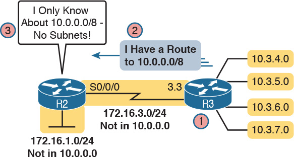
Let’s follow the steps in the figure:

1. R3 has autosummary enabled, with the EIGRP auto-summary router subcommand.

2. R3 advertises a route for all of Class A network 10.0.0.0, instead of advertising routes for each subnet inside network 10.0.0.0 because the link to R2 is a link in another network (172.16.0.0).

3. R2 learns one route in network 10.0.0.0: a route to 10.0.0.0/8, which represents all of network 10.0.0.0, with R3 as the next-hop router.

Example 10-16 shows the output of the show ip route command on R2, confirming the effect of the auto-summary setting on R3.

Example 10-16 R2 with a Single Route in Network 10.0.0.0 for the Entire Network

Click here to view code image

---

R2# show ip route eigrp
! lines omitted for brevity

D     10.0.0.0/8 [90/2297856] via 172.16.3.3, 00:12:59, Serial0/0/0

---

Note that auto-summary by itself causes no problems. In the design shown in Figure 10-9, and in the command output in Example 10-16, no problems exist. R2 can forward packets to all subnets of network 10.0.0.0 using the one highlighted summary route, sending those packets to R3 next.

To better understand what the terms contiguous and discontiguous mean in networking, refer to the following two formal definitions when reviewing the example of a discontiguous classful network that follows:

Contiguous network: A classful network in which packets sent between every pair of subnets can pass only through subnets of that same classful network, without having to pass through subnets of any other classful network

Discontiguous network: A classful network in which packets sent between at least one pair of subnets must pass through subnets of a different classful network

Figure 10-10 creates an expanded version of the internetwork shown in Figure 10-9 to create an example of a discontiguous network 10.0.0.0. In this design, some subnets of network 10.0.0.0 sit off R1 on the left, whereas others still connect to R3 on the right. Packets passing between subnets on the left to subnets on the right must pass through subnets of Class B network 172.16.0.0.

Autosummarization causes problems in that routers like R2 that sit totally outside the discontiguous network become totally confused about how to route packets to the discontiguous network. Figure 10-10 shows the idea, with both R1 and R3 advertising a route for 10.0.0.0/8 to R2 in the middle of the network. Example 10-17 shows the resulting routes on Router R2.

Example 10-17 R2 Routing Table: Autosummarization Causes Routing Problem with Discontiguous Network 10.0.0.0

Click here to view code image

---

R2# show ip route | section 10.0.0.0
D     10.0.0.0/8 [90/2297856] via 172.16.3.3, 00:00:15, Serial0/0/0
                 [90/2297856] via 172.16.2.1, 00:00:15, Serial0/0/1

---

As shown in Example 10-17, R2 now has two routes to network 10.0.0.0/8: one pointing left toward R1 and one pointing right toward R3. R2 simply uses its usual load-balancing logic, because as far as R2 can tell, the two routes are simply equal-cost routes to the same destination: the entire network 10.0.0.0. Sometimes R2 happens to forward a packet toward the correct destination, and sometimes not.

This problem has two solutions. The old-fashioned solution is to create IP addressing plans that do not create discontiguous classful networks. The other: Just do not use autosummary, by using EIGRP defaults, or by disabling it with the no auto-summary EIGRP subcommand. Example 10-18 shows the resulting routing table in R2 for routes in network 10.0.0.0 with the no auto-summary command configured on Routers R1 and R3.

Example 10-18 Classless Routing Protocol with No Autosummarization Allows Discontiguous Network

Click here to view code image

---

R2# show ip route 10.0.0.0
Routing entry for 10.0.0.0/24, 8 known subnets
  Redistributing via eigrp 1
D        10.2.1.0 [90/2297856] via 172.16.2.1, 00:00:12, Serial0/0/1
D        10.2.2.0 [90/2297856] via 172.16.2.1, 00:00:12, Serial0/0/1
D        10.2.3.0 [90/2297856] via 172.16.2.1, 00:00:12, Serial0/0/1
D        10.2.4.0 [90/2297856] via 172.16.2.1, 00:00:12, Serial0/0/1
D        10.3.4.0 [90/2297856] via 172.16.3.3, 00:00:06, Serial0/0/0
D        10.3.5.0 [90/2297856] via 172.16.3.3, 00:00:06, Serial0/0/0
D        10.3.6.0 [90/2297856] via 172.16.3.3, 00:00:06, Serial0/0/0
D        10.3.7.0 [90/2297856] via 172.16.3.3, 00:00:06, Serial0/0/0

---

feasible distance

feasible successor

reported distance

successor

unequal-cost load balancing

variance

autosummary

discontiguous network