Chapter 10: Working with Network Address Translation

While commonly referred to as Network Address Translation (NAT), this term covers both NAT and Port Address Translation (PAT). In this chapter, we will learn how to use NAT (and PAT) to ensure that our traffic can reach its destinations. We will explore both automatic and manual NAT options. Additionally, we will see when the use of static or dynamic NAT is appropriate and look at a few specific cases where additional configuration in Gaia might be required to achieve the desired address translation. As you read about various configuration examples, you’ll be instructed to either apply the relevant ones to our lab or not, for those that are used for demonstration and explanation. While NAT is a universal subject in networking, it is important to understand Check Point’s implementation specifics.

In this chapter, we are going to cover the following main topics:

• The need for NAT
• NAT policies, rules, and processing orders
• Automatic NAT use cases and behaviors
• When NAT is not enough
• NAT logging configuration and interpretation

The need for NAT

NAT is most commonly used to circumvent the problems caused by the shortage of public IP addresses. Due to the exhaustion of public IPv4 addresses, private networks predominately use IPv4 addresses defined in RFC 1918 (RFC, or Request for Comment, being the form of publication for the development and adoption of standards of communication for the internet). These are comprised of the following ranges:

Table 10.1 – The RFC 1918 IPv4 address ranges and networks

These addresses are reserved for use in private environments that are isolated from one another. Traffic to external services hosted on the internet from these ranges (and the networks they are comprised of) should either be translated into public IP addresses or be discarded by the upstream routers.

Conversely, services hosted in private networks usually reside on hosts with private IP addresses. To make these services accessible from the outside, they are statically translated into specific public IP addresses. Then, these public IP addresses are used in publicly accessible DNS records to direct inbound traffic to the networks that the external interface(s) of your gateways or clusters are connected to. NAT is then used to replace the public IP address with the private IP address assigned to a host (or a load balancer).

Another use case for NAT is the merging of private networks. During mergers and acquisitions, a situation might arise where multiple environments are comprised of either identical or overlapping networks. To merge such infrastructures, these conflicts must be resolved. Either some of those networks must be renumbered (which is a complex and intrusive process with downtime), or NAT can be used between them.

Yet another case that is similar to the previous one is VPN connectivity between organizations with overlapping encryption domains (as encryption domains are often comprised of the networks from RFC 1918). If such situations are encountered, peers can supply each other with non-conflicting addresses or ranges that can be used to translate the sources.

An additional upside to the use of NAT is obfuscation of the private hosts and networks behind the addresses they translate to, allowing for egress traffic to reach its destinations but preventing connectivity in the opposite direction.

With the NAT use cases covered, in the next section, let’s take a look at NAT policies, rules, and processing orders.

NAT policies, rules, and processing orders

With each new policy package, a NAT policy is automatically created. When we click on it in the navigation view on the left-hand side, we can see that it is comprised of the following column headers:

• No.
• Name
• Original Source
• Original Destination
• Original Services
• Translated Source
• Translated Destination
• Translated Services
• Install On
• Comments

Right-clicking anywhere in the headers area will manifest a column selector menu where we can check an empty checkbox for Hits to enable counters for each rule:

Figure 10.1 – The NAT policy structure

A policy is prepopulated with several section titles prefixed with Automatic Generated Rules:, and followed by either (No Rules) or the rule numbers within the section.

These are listed as follows:

• Machine Static NAT
• Machine Hide NAT
• Address Range Static NAT
• Network Static NAT
• Address Range Hide NAT
• Network Hide NAT
• Manual Lower Rules

Right-clicking on either the top or the bottom one of these section titles will reveal an option to create new rules either above or below the automatically generated rules.

NAT rules are processed top-down, and up to two rules can be applied to traffic; for example, one rule can cover the source and another rule can cover the destination address translation.

Manual rules that are created above the automatic NAT rules should be used for either exceptions from the address translations or for specific address and service translations.

Manual rules located below the automatic rules should be used for cases not covered by the automatically generated rules.

NAT is direction-dependent. Traffic traversing our gateways or clusters is modified either before it is routed or after, to achieve the desired behavior. To visualize the process, let’s look at the following diagram. We can see that when packets are moving from left to right [1], Destination NAT [2] is applied prior to Gaia IP Routing [3] and Source NAT [4] is applied after the routing:

Figure 10.2 – The source and destination NAT options relative to routing

Alternatively, to see where NAT is taking place relative to the access control policy rules, VPNs, and Gaia IP routing, take a look at the following diagram:

Figure 10.3 – The source and destination NAT options relative to other modules

Note that not all the actions depicted in the preceding diagram are necessarily taking place. Only selected options in a specific direction are enforced. Packets must be allowed by Anti-Spoofing and the rule in the Access Control policy; hence, they are shown as checked.

The simplest, if somewhat limited in its capabilities, way to implement NAT is to rely on an automatic NAT rule provisioning mechanism.

Automatic NAT

Automatic NAT is configured in the properties of objects. Each time NAT is defined in the properties of a gateway/cluster, management server, host, network, or range, several rules for each object are automatically created in the corresponding Automatic Generated Rules sections.

We should bear in mind that since we are working in a single security domain with the common objects database, once NAT has been configured for an object, the corresponding automatic rules will be identical in all the policy packages we might create.

Automatic static NAT

Static NAT refers to the consistent translation of hosts’ original IP addresses into specific addresses. Let’s take a look at a few example implementations next.

One-to-one

Automatic static NAT is defined in a host object and performs one-to-one NAT, translating the actual IP address of the object into the address we would like it to be accessible by from the networks behind different interface(s) of the firewall.

One common scenario is an assignment to host object [1] with NAT properties [2] configured to Add automatic address translation rules [3], the Translation method option configured as Static [4], and the Translate to IP address value defined as one of the public IPs from the network on the external interface of the gateway or a cluster [5]. For static NAT, we should choose the target in the Install on gateway field [6]:

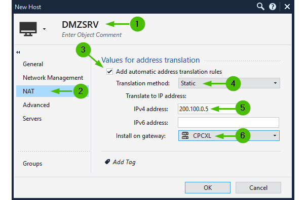
Figure 10.4 – Automatic static NAT for the host object

Note

Configure the DMZSRV object in our lab, as shown in the preceding screenshot.

For the management server(s) to manage remote gateways and receive logs from those devices, we must assign it a public IP address, too.

In the properties of the management server [1], go to the NAT section of the navigation tree [2]. With Add Automatic Address Translation rules selected [3], choose Static [4], and in Translate to IP Address | IPv4 Address, type in the public IP address indicated in our lab topology diagram (200.100.0.10) [5]. In Install on Gateway, click on the ellipsis (…) and select the CPCXL cluster object [6]. Check the box for Apply for Security Gateway control connections [7] to ensure that we’ll be presenting this public IP to the remotely managed gateways:

Figure 10.5 – Automatic static NAT for the management server

Note

Configure the CPSMS object in our lab, as shown in the preceding screenshot.

Many-to-many

There are situations where a one-to-one NAT should be performed for either the range of addresses or an entire network to preserve the individual addressability of each NATed host.

If we have to translate an entire network, follow these steps. In the properties of the Network object, select the Static NAT and specify the corresponding address of the desired NAT network:

1. To achieve this, open the Network object [1], and in its NAT properties, check the Add automatic address translation rules box [2]. Then, choose Static as the Translation method option [3], and specify the network for correlated many-to-many translation in the IPv4 address field [4]. In Install on gateway, choose the desired gateway or a cluster [5]:

Figure 10.6 – Automatic static NAT for a many-to-many scenario

This will automatically create the corresponding rules and allow automatic static translation of each source IP address to the aligned IP in the target (Translate to IP address) network, that is, 10.10.10.1–192.168.100.1 to 10.10.10.254–192.168.100.254.

Note

Do not configure this in the lab.

If this configuration is already present and active, the resultant traffic logs [1] will indicate the preservation of the last octet [2] when translated [3], along with the current number of the automatically generated NAT rule [4]:

Figure 10.7 – The automatic static NAT log for a many-to-many scenario

2. If a many-to-many static NAT is performed on a range of IP addresses [1], set the NAT properties [2] to automatic [3], choose Static [4] as the translation method, type in the IPv4 address from which the one-to-one correlation will start [5], and select the installation target [6]:

Figure 10.8 – Automatic static NAT for a range of IP addresses

In Figure 10.8, the 10.10.10.20 IP address will be translated into 192.168.111.20 and so on.

Note

Do not configure this in the lab.

Single host hiding behind a unique IP address

Let’s configure a host object [1] called SmartConsole_VM [2] with NAT properties [3] for automatic NAT [4]. Select the translation method as Hide [5], choose Hide behind IP address [6], specify the public IP address (200.100.0.20) [7], and select our cluster as the installation target [8]:

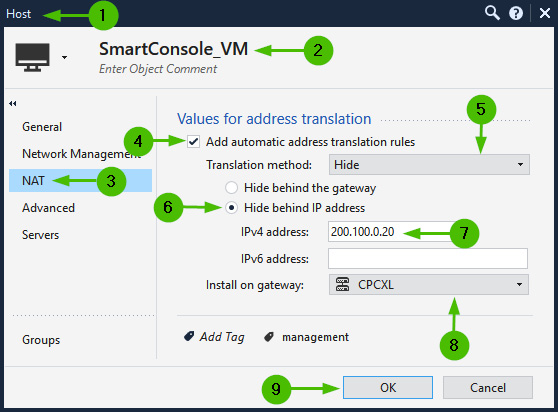
Figure 10.9 – Static hide behind IP address NAT configuration

Note

Configure the SmartConsole_VM object’s NAT in our lab, as shown in the preceding screenshot, for consistent egress traffic origin.

Regardless of the destination, whether external (the internet), internal (the networks behind other interfaces), or DMZ, our source IP will always be translated to that which is specified in the Hide behind IP address properties.

This might not always be desirable behavior. We’ll address how to limit hide NAT to only the external connections shortly.

Automatic dynamic NAT

The most frequently encountered type of address translation that can be found in every home router’s out-of-the-box configuration is when all IPs behind the router’s internal interfaces are translated into a single public IP address assigned by the ISP.

When we are talking about dynamic NAT, we are indeed touching on the subject of PAT, so the subject of NAT pools should now be mentioned.

Source port pools

Check Point uses the ports Pool feature to multiplex the use of identical source ports if any of these parameters in address translation are different: IP protocol, Hide source IP, or Destination IP. To learn more about this feature, see sk156852 “NAT Hide failure - there are currently no available ports for hide operation. Please refer to sk156852.” error in SmartConsole / SmartLog / SmartView Tracker. In total, Check Point uses approximately 50,000 “high” ports (those between 10,000 and 60,000).

In gateways with less than eight CPU cores or six CoreXL FW instances (we learned about CoreXL SND and CoreXL FW instances in the Packet flows and acceleration section of Chapter 8, Introduction to Policies, Layers, and Rules), the entire range of ports used for NAT is statically divided between these instances. If we are to execute cpview and navigate to Advanced | NAT | Pool-IPv4 [1], then in the High port section [2], we can see the top two used pools [3] and their capacities [4] being close to 50K divided by the number of CoreXL FW instances (our four-core gateway has one CoreXL SND instance and three CoreXL FW instances):

Figure 10.10 – The NAT pool with GNAT disabled (unit with four CPU cores)

Larger gateways with more than eight CPU cores (or more than six CoreXL FW instances) are automatically configured to use the Global NAT (GNAT) feature, which utilizes the global NAT ports allocation table.

For some reason, gateways with less than eight CPU cores have that feature disabled by default. I’m not sure what the reason for that is, since it is explicitly stated in sk164155 Dynamic Balancing for CoreXL that on models with fewer than eight cores, you must enable a GNAT port allocation feature.

To do that, let’s check whether GNAT is already enabled by running fw ctl get int fwx_gnat_enabled in expert mode. If it is not running (fwx_gnat_enabled = 0), enable GNAT by appending the fwx_gnat_enabled=2 line to fwkern.conf located in $FWDIR/boot/modules/ and rebooting the gateway.

Once rebooted, the size of the pool for each source/destination pair is close to 50,000. If we are to execute cpview and navigate to Advanced | NAT | Pool-IPv4 [1], in the High port section [2], we can see the top two used pools [3] and their capacities [4] being close to 50K:

Figure 10.11 – Port pools with GNAT enabled

Now that we’ve seen how the ports are allocated for dynamic NAT, let’s look at the number of ways the automatic dynamic NAT can be configured.

Automatic many-to-one (hide behind NAT)

Hide behind, also referred to as many-to-one NAT. In Check Point, we can use three ways of implementing it:

• Hide internal networks behind the gateway’s external IP in the gateway/cluster properties.
• Hide internal networks, ranges, or hosts behind the gateway’s IP in the objects’ properties.
• Hide internal networks, ranges, or hosts behind the specific IP in the objects’ properties.

Hiding internal networks behind the gateway’s external IP

In most rudimentary environments, private IP addresses located behind internal (or DMZ) interfaces of the firewalls are hidden behind public IP addresses assigned to the external interface of a single gateway or as a virtual IP address of a cluster.

While this is the easiest option to configure, it should be used judiciously. I would recommend it for the smallest environments, such as retail or banking branches with no more than 50 IPs behind the gateway/cluster.

This option is disabled by default. It can be enabled in Gateway Cluster Properties, in the NAT section, by checking Hide internal networks behind the Gateway’s external IP:

Figure 10.12 – Hide internal networks behind the Gateway’s external IP

Note

Do not configure this in the lab.

In this case, our internet-bound traffic is NATed, while the traffic between the internal networks and hosts is not. The log details for the outbound connections [1] would indicate that our source IP address is translated into that of our cluster [2] and that the NAT Rule Number field is 0 [3]. This rule is invisible in the NAT policy and is superseded by any other more specific rule:

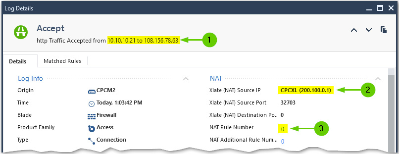
Figure 10.13 – Hiding internal networks behind the gateway’s external IP log

Hiding internal networks, ranges, or hosts behind the gateway’s IP

This option gives us slightly more flexibility, as we might choose specific networks, ranges, and hosts that require access to the internet and, thus, should be subjected to NAT.

As shown in the following screenshot, in the Net_10.20.20.0 network object [1], select NAT [2]. Then, choose automatic address translation [3], select Hide for Translation method [4], choose Hide behind the gateway [5], and select our cluster as the installation target [6]:

Figure 10.14 – Dynamic NAT for a network (or a range) object; hide behind the gateway

Note

Configure the Net_10.20.20.0 and Net_10.10.10.0 objects in our lab, as shown in the preceding screenshot.

Note

If we are using the Hide behind the gateway NAT option, Install on gateway might remain at the * All default setting. This could be relevant if you are using internal routing for egress traffic redundancy.

In this case, traffic originating from this object will always be translated into the IP address of the gateway/cluster interface closest to the destination. As shown in the following screenshot, when we are accessing resources on a different internal network [1], our source is translated into the virtual IP of the cluster in the destination’s range [2]. When we are reaching out to the internet [3], our source IP is translated to the external IP of the cluster [4]. In both cases, the same NAT Rule Number, 9, is in effect [5]:

Figure 10.15 – Hiding behind the gateway in the objects’ properties logs

Hiding internal networks or ranges behind specific IP addresses

This is similar to the Hide behind the gateway option but allows for added flexibility. There is a good reason not to hide your internal networks behind your gateway’s or cluster’s public IPs. Consider the possibility that either one or several of your hosts have been compromised and, despite your best efforts, generate malicious traffic. In this case, the public IP address associated with it will likely be blocked upstream. If that IP is the same as the external interface of your gateway, its functionality might be negatively affected.

Another compelling reason for this is possible port exhaustion, which happens if the capacity of the Source Port Pool instance has been exceeded. If you have a sufficiently large public IP range or a connected network on your external interfaces and if your internal networks are relatively small (like Class C), you can configure each of the internal networks [1] for automatic NAT [2] hiding them [3] behind individual public IP addresses [4] on a specific gateway or a cluster [5], as shown in the following screenshot:

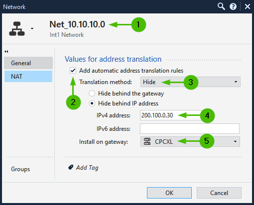
Figure 10.16 – Hiding internal networks or ranges behind specific IP addresses

Note

Do not configure this in the lab.

This will increase the capacity for the dynamically allocated hide NAT ports.

The same approach could be used for the IP ranges’ NAT properties.

Preventing unnecessary NAT

While it makes sense to translate addresses for outbound or inbound access to and from the internet, in most cases, traffic inside the environment protected by the gateway or a cluster should remain untranslated.

To prevent unnecessary NAT between the internal and DMZ hosts, we should create a Network Group object [1], name it Int_Nets [2], and add all our internal and DMZ networks to it [3]. Save the object and, in our NAT policy, create a rule at the top [4] called No NAT. Add the newly created Int_Nets group to both the Original Source and Original Destination fields [5]:

Figure 10.17 – Preventing NAT inside our environment

Note

Create the Int_Nets group, and create the No NAT rule in the lab.

This will restrict NATed traffic to the external interface of the gateway using the virtual IP address of the external cluster interfaces, or the specific IP addresses indicated in the Hide behind IP address fields.

Now that we have seen the possibilities afforded by automatic NAT defined in the properties of the objects, let’s take a look at how more complicated tasks involving NAT and PAT could be accomplished.

When NAT is not enough

While the majority of cases in simple and small environments can be handled by automatic NAT defined in objects’ properties, with increasing scale and complexity, we will have to resort to manual NAT rules.

Note

The information in this section should be used for reference only since it requires the presence of an access control policy, which we have not yet created.

Let’s look at a few more complex examples of manual NAT implementation that, in addition to the creation of NAT rules, might require a few Gaia configuration changes.

Many-to-less

If your internal networks are larger than Class C, using the Hide behind IP address option described in the previous section might not be feasible. You can still do that by representing your large network as several ranges, each with its own public IP in the NAT properties, but this is a rather tedious process.

An alternative way to handle this issue with greater flexibility is with the following steps:

1. Create a new manual rule at the bottom of the NAT policy under the Manual Lower Rules section title.
2. Create a Network Group object for your source networks requiring outbound access to the internet (for example, we can use our Int_Nets group) and place it in the Original Source field of the new manual NAT rule. Create a new Address Range object [1], naming it appropriately [2], and define the scope of unused IP addresses from your public range or a network [3]:
   

Figure 10.18 – Creating an IP range to use as a hide NAT translated source

3. Place this object in the Translated Source field of our rule. You should now see this object with a small red S letter, indicating that the preset NAT mode is static [1]. Right-click on it, click on NAT Method [2], and click on Hide [3]:

Figure 10.19 – NAT Method change from Static to Hide

4. Once done, the red S character is changed to H, and the rule should look like this:

Figure 10.20 – Setting manual NAT rule to Hide behind address range

Now things are about to get a little bit complicated… For each automatically created NAT rule with either Static or Hide behind the IP address options, the background process creates a proxy ARP record. A proxy ARP record is an association of the translated IP address with the MAC address of the gateway’s (or cluster members’) interface, and the actual IP address of that interface. We can look those up for the objects we have configured by executing the fw ctl arp -n command in the Expert mode of our gateway (in our case, each cluster member). I am using another command, clish -c "show cluster state" | grep local, for the compact illustration of active and standby cluster member states.

Figure 10.21 – Automatic proxy ARP records

The output is comprised of the NAT IP address, the MAC address of the interface it is associated with, and the IP address of that interface configured on the gateway (or a cluster member).

For our rule to go into effect, we have to create individual proxy ARP records for each IP address in the Hide_NAT_Range object.

To accomplish this, we must perform the following steps:

1. Make a change in the Global Properties dashboard’s [1] NAT section [2] by checking the Merge manual proxy ARP configuration box [3] and clicking on OK [4]:

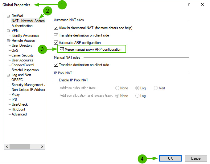
Figure 10.22 – The Global Properties Merge manual proxy ARP configuration option

2. Publish the changes and install the policy.
3. Log into each cluster member via SSH, and in CLISH, enter the following commands:
   • For CPCM1, enter the following:

     add arp proxy ipv4-address 200.100.0.40 interface eth4 real-ipv4-address 200.100.0.2

     add arp proxy ipv4-address 200.100.0.41 interface eth4 real-ipv4-address 200.100.0.2

     save config

   • For CPCM2, enter the following:

     add arp proxy ipv4-address 200.100.0.40 interface eth4 real-ipv4-address 200.100.0.3

     add arp proxy ipv4-address 200.100.0.41 interface eth4 real-ipv4-address 200.100.0.3

     save config

4. Install the policy again.

Now, we can verify that new proxy ARP entries are in effect:

Figure 10.23 – The proxy ARP entries with IPs from the Hide_NAT_Range object

If we remove the Hide behind the gateway settings from our two internal network objects and install the policy again, we’ll be using IPs from the Hide_NAT_Range object.

Manual static NAT

If (in addition to the IP translation) we must rely on port translation, automatic NAT will be of no help, as the rules created by defining NAT in the properties of the objects are not editable. In this case, we must create an additional object with the public (or translated) IP address and create associated proxy ARP records for it on relevant interfaces*.

*

Proxy ARP entries are only necessary if we are translating to IP addresses in connected networks. If your public IP range does not reside on a connected network of your external interfaces (for instance, when the ISP provides you with an additional small range used between your gateways and their own equipment), proxy ARP entries are not required.

For example, for a WebSrvPrivate web server object with an IP of 10.30.30.100 listening on port 5080, we should create a WebSrvPublic object with an IP address of 200.100.0.100 and one proxy ARP record added on each cluster member.

On CPCM1, use the following:

add arp proxy ipv4-address 200.100.0.100 interface eth4 real-ipv4-address 200.100.0.2

save config

On CPCM2, use the following:

add arp proxy ipv4-address 200.100.0.100 interface eth4 real-ipv4-address 200.100.0.3

save config

Then, the pair of NAT rules for outbound and inbound traffic must be created:

Figure 10.24 – The manual static NAT rules for service translation

Additionally, the accompanying access control rule allowing the http traffic from ExternalZone to WebSrvPublic needs to be created:

Figure 10.25 – The access control policy rule for the manually NATed server

With these steps completed, we should install the policy.

The server is now accessible [1], and traffic from the External zone [2] on the HTTP service [3] addressed to the public IP of the server [4] is being translated to the correct destination [5] and port 5080 [6]:

Figure 10.26 – The access control rule log for manual static NAT with service translation

An additional edge case is applicable in very small environments where you have a small gateway with a single public IP address. In this situation, you can create an object with the same public IP address as the one assigned to the external interface of your gateway, use public DNS to redirect traffic to the high port, and use manual static NAT to translate it to the service running on the desired port on internal or DMZ networks.

In this case, no proxy ARP configuration is required, as the IP address being used is already associated with the interface.

NAT pools

Occasionally, you might have to deal with situations where some of your peer organizations require you to source your connections from specific IPs or networks. To accomplish this, you can either create an actual network to accommodate the peer or you can use NAT pools.

Individual NAT pools are created in Gaia WebUI Advanced Routing | NAT Pools.

The Add NAT Pool [1] window contains the following fields: a Destination field [2] and a Subnet mask field [3]. We can use networks or individual hosts (with the /32 mask):

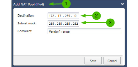
Figure 10.27 – NAT pools

In a cluster, identical pools must be defined for all members. These pools can then be advertised as regular networks via routing protocols to the upstream router or routers might be preconfigured with static routes for specific NAT pools using our firewalls or clusters’ actual IP as the gateway.

We can now use addresses from NAT Pool in the Hide behind IP address fields for our hosts or networks initiating a connection to that peer.

Bells and whistles

So far, all the cases we’ve looked at are relatively simple but necessary to understand. To get a better idea about Check Point’s NAT policy capabilities, let’s look at the NAT policy in the demo mode:

Figure 10.28 –The NAT policy in demo mode

As we can see, in addition to the examples of hosts, networks, and ranges that we had to work with, dynamic objects [1], access roles [2], FQDN domains [3], zones [4], and updatable objects [5] can be used in manual rules, providing great flexibility in traffic handling. Services can be conditionally redirected [6] and, of course, PAT can be used with all of these by populating the Original Services and Translated Services fields in the rules.

While we have discussed logging in general and have mentioned NAT logging in passing, let’s spend a minute on NAT-specific log entries in the event log cards.

NAT logging

NAT is logged in rules where Log Generation | Per Connection are enabled. As per the recommendations made in Chapter 8, Introduction to Policies, Layers, and Rules, this should be the default setting for the firewall-only rules.

The NAT portion of the log card is really easy to understand, but I have seen repeated questions in forums regarding these two fields: NAT Rule Number and NAT Additional Rule Number.

To illustrate, let’s take a look at the following log card:

Figure 10.29 – The NAT Rule Number and NAT Additional Rule Number log fields

In the preceding screenshot, we can see the following:

• Traffic is accepted from host 10.10.10.21 [1] to host 200.100.0.5 [2].
• The translated source IP is 10.30.30.1 [3], which belongs to one of the virtual IPs of our cluster, and the translated destination is 10.30.30.5 [4].
• We can see that NAT Rule Number is 4 [5] and NAT Additional Rule Number is 9 [6].

This log describes the scenario where the DMZSRV object is being accessed from inside by its public IP from the network configured to Hide behind the gateway. NAT is performed on both; the destination [1], source [2], and corresponding rule numbers are shown here:

Figure 10.30 – The NAT Rule Number and NAT Additional Rule Number rules

If only one translation is taking place, we will see either the Xlate (NAT) Source IP field or the Xlate (NAT) Destination IP field. The other one will be suppressed. In such a case, only Nat Rule Number will have the rule number value and NAT Additional Rule Number will have 0 in it.

Summary

In this chapter, we learned how to work with NAT policies, rules, and methods. We covered the automatic static and dynamic NAT capabilities of different objects and saw how they could be applied and logged. We learned about cases requiring manual NAT rules alongside additional Gaia configurations that might be necessary to accommodate more complex NAT scenarios in our data centers. As we went through this chapter, we configured NAT properties for the objects in our lab.

In the next chapter, using objects created in this and the previous chapters, we’ll be creating and working with our first access control policy.