
Chapter 22. Metric-Driven Cost Optimization
Metric-driven cost optimization (MDCO) is the driver that measures potential optimizations and then uses goals and target lines to trigger an operate process to action them. When you are buying commitments, you’re in the operate phase. With MDCO, you use the metric threshold to determine precisely when you take those actions.
MDCO could also be described as “the lazy person’s approach to cloud cost management.” The primary rule of MDCO is: don’t do anything. That is, don’t do anything until you have a metric that measures the impact of your actions. If you make optimizations but don’t have metrics to tell you whether they’ve been positive or negative on your spending, you’re not doing MDCO.
By the end of this chapter you’ll know how to use metrics to correctly drive your cost optimizations.
Core Principles
There are a few core principles that define the MDCO practice:
- Automated measurement
- Computers perform the measuring, not humans.
- Targets
- Metrics without targets are just pretty graphs.
- Achievable goals
- You need a proper understanding of data to determine realistic outcomes.
- Data driven
- Actions aren’t driving your data: the data is driving you to take actions.
We’ll explain each of these principles throughout this chapter.
Automated Measurement
Loading billing data, generating reports, and generating recommendations for optimizations are all tasks that should be done by automation, or via a FinOps platform. When massive amounts of billing data is delivered by your cloud service provider, all of these activities need to kick off automatically. Having FinOps practitioners trying to run ad hoc data processing and report generation slows down MDCO and will result in slow responses to anomalies.
Repeatable and reliable processing of the data allows you to remain focused on the real task at hand: saving money. You can then spend time refining the processes being followed and working on more deeply understanding the cost optimization programs and how they are reflected in the data/metrics.
Targets
For MDCO, target lines are key. We wrote in Chapter 14 about how target lines give more context to graphs. We’ve always been firm believers that no graph should be without a target line. Without it, you can determine only basic information about the graph itself, not what the graph means for your organization. The target line creates a threshold from which you can derive a trigger point for alerts and actions.
Tip
Humans don’t do well understanding the scale of very large numbers, which is why contextual targets are so important. To counteract this, a tip from Hans Rosling’s book Factfulness (Flatiron Books, 2020) was quoted by Anders Hagman from Spotify at a recent FinOps Foundation monthly summit. In the book, Rosling tells readers that “whenever someone gives you a large number, ask for another number” to measure it against. In MDCO, for your metrics to provide value, you need a target to measure against.
Achievable Goals
There are several metrics to monitor across cost optimization programs. Having each metric correctly tracked enables the operational strategies for your cost optimizations. Every individual optimization will have a different impact on your savings realized, so you shouldn’t treat all optimizations as equal. When combining metrics, you should be normalizing the data based on the savings potential of the optimization.
One of the most common incorrectly measured metrics, and one that can help you understand achievable goals in MDCO, is commitment coverage.
There are multiple ways to measure cost optimization performance, and each method represents a particular view on efficiency. Depending on the method you use, 100% optimization may not be achievable. For MDCO, measurements that are completely achievable are required to determine the right time to perform actions.
Let’s work through commitment coverage to explain this in more detail.
Commitment coverage
Commitment coverage is the metric that shows how much usage is being charged at on-demand rates versus discounted rates. Generally, organizations set a target coverage—commonly, it’s 90%. Let’s compare the various methods.
In the traditional model, you measure coverage by counting up all the commitment hours that you have and then dividing that number by the total hours you ran in the period (see Figure 22-1).

Figure 22-1. Commitment coverage calculated via raw hours
Even though the way coverage is measured in Figure 22-1 is correct, this may not be the right way to do it. With elastic infrastructure, resources come and go frequently, and there are some hours that shouldn’t be covered by a commitment because there simply isn’t enough usage during the period of time to warrant it. Ideally, you don’t include all the usage that is under the break-even threshold, below which commitments would cost more than they save. By removing these noncoverable hours, you can measure coverage over coverable hours (see Figure 22-2).
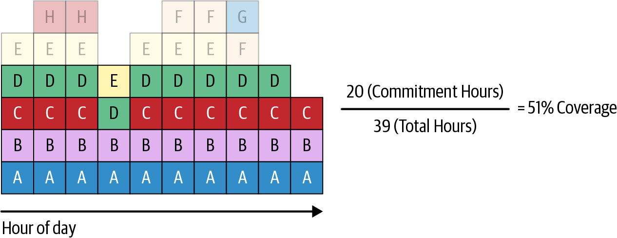
Figure 22-2. Commitment coverage calculated via coverable hours
If you remove noncoverable hours that shouldn’t be covered at the peaks in the graph (those indicated as H, F, G, and E in Figure 22-2), you get a clearer picture of the true coverage percentage. A and B are covered by a commitment, leaving the hours covered by resources C, D, and E at on-demand rates. Buying an additional two commitments provides 100% coverage, and the two extra commitments would save money.
So far, you’ve been treating the cells in the graphs as if they are all the same thing: B is the same as A, which is the same as C. But in reality, each cell (or hour or second) may be a wildly different-sized usage. Usage marked as A may cost over $1 an hour, while B may cost $0.25 an hour. The amount you save on each commitment would then be vastly different. Primarily, you buy commitments for savings, so measuring them as consistent blocks—when they are so different—provides misleading results. The goal is to work out how much of your coverage is actually generating savings.
Converting the hour cell into possible savings by covering it with a commitment clearly shows the effect of a commitment on your cloud bill. Adjusting the graph by the relative savings of each usage type, you end up with a very different picture (see Figure 22-3).
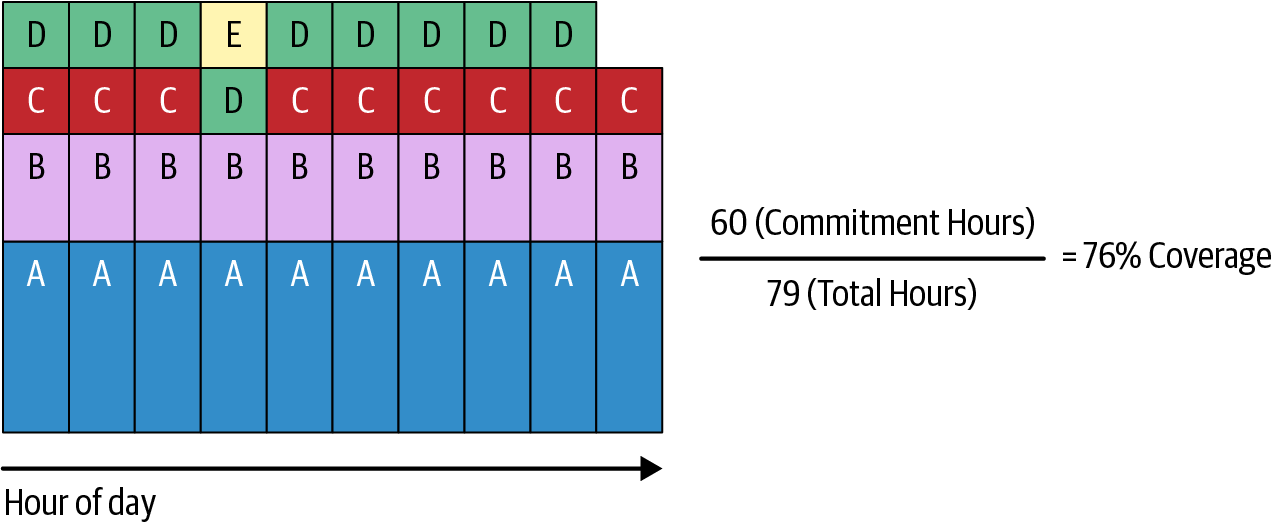
Figure 22-3. Commitment coverage calculated via weighted coverable hours
Figure 22-3 shows that you’re actually closer to 76% of achievable savings. The original assessment in Figure 22-1 showed you as being in a very low-coverage situation. But the new weighted position, which also removes hours that shouldn’t actually be committed, shows that your position isn’t really that bad.
The key takeaway is that committing different resources realizes different amounts of savings. Not all usage is coverable, so including it all in committed coverage results in metrics that are more difficult to set targets against. However, by thinking in terms of achievable coverage, you can more accurately determine how and where to make improvements.
Savings metrics that make sense for all
Adding up the savings across everything that should be committed gives you a concept of total potential savings. For example, let’s assume all of the cells in Figure 22-3 would save $102,000 per year when covered with a commitment (total potential savings). So, 76% of the $102,000 is the amount of savings currently being realized (realized savings), leaving the remaining 24% uncovered and at the on-demand rates (unrealized potential savings).
This connects back to the language of FinOps. When you move away from talking about usage hours and commitment coverage rates to a place where the conversation is “you are currently realizing 76% of your total potential savings of $102,000,” this conveys to everyone in the organization where you stand and where you could go. Further, it removes the need for a deep understanding of the intricacies of commitment-based discounts and enables conversations within the organization. You’ve created a common lexicon for mutual understanding.
Combining metrics
To determine a performance metric for your commitments, you measure how much of a commitment is being used versus not being used over a specific time period. This is called your commitment utilization. At an individual commitment level you monitor by time, measuring the proportion of hours (or seconds) that a commitment applied a discount to your resource usage versus the number of hours (or seconds) you didn’t have any usage for the commitment to discount.
However, if you roll your commitment utilization up to show one overall performance metric, the individual underperforming commitments can be hidden. Instead, you measure individual commitments and alert when they individually underperform. Let’s look at an example of this in Figure 22-4.

Figure 22-4. Commitment usage over time
You use the usage in Figure 22-4 to determine your commitment utilization, based on having seven commitments. You can see that the first four commitments are utilized 100%. The fifth commit will have 90% utilization and the sixth will have 80% utilization, with the last commitment at only 50%.
If you just average out the utilizations (100% + 100% + 100% + 100% + 90% + 80% + 50%) / 7, you get 88.5% utilized. An overall utilization rate of 88% on the surface appears pretty decent and wouldn’t raise concerns. Had you set a target utilization of 80%, MDCO would reflect no changes needed. But remember: there’s an individual commitment achieving only 50% utilization, and that deserves your attention and possible modification.
Data Driven
For years, teams have been operating their services using metrics to monitor items like service performance, resource usage, and request rates as an early warning system, alerting the teams when thresholds are passed or events triggered and consequent adjustments are needed.
Operating FinOps optimizations without metrics provides no real method of identifying when optimizations are meeting goals. In fact, without metrics you can’t even set goals. The tracked metrics build upon the feedback loop we discussed in Chapter 9. Metrics help you identify where you’re unoptimized or underperforming so you can make improvements. In other words, metrics help you measure how much your cost optimizations are saving.
Applying MDCO to FinOps allows you to measure the desired outcomes of a cost optimization. When metrics show that a change has not been successful, you can use this as an early warning that the change needs further adjustment, or you can roll it back entirely.
Tip
In Episode 11 of the FinOpsPod, TJ Johnson from Box.com explained how most visualizations in FinOps help you answer four main questions that tie nicely with an MDCO approach, though he uses some slightly different terminology:
How am I doing so far? Measurement of where you are currently.
How do I get better? Identifying the optimizations you can make and helping you select which areas you would like to tackle.
Am I actually getting better? Measuring how you are improving over time, forming a set of key momentum indicators (KMI), which help you monitor if you are getting better—or worse—over time.
Have I reached my goal? Providing feedback on when you are completing the goals you have previously set.
Measurements that answer these four questions play into a DevOps mindset, where there’s constant data flowing in to feed into the decision making of the application team, the finance team, and the business. Listen to the episode to get the full story of how he does it at Box.com.
Metric-Driven Versus Cadence-Driven Processes
In Chapter 18, we discussed strategies around commitment-based discounts. Most companies, when starting out with commitments, will purchase their commits on a schedule (monthly, quarterly, or even yearly). We call this cadence- or schedule-driven cost optimization.
If you purchase in slow cycles, you end up with large amounts of uncovered usage. Figure 22-5 shows some usage over time, and in dark gray you see the commitment coverage you have. You can see from the graph that purchases of commits are occurring on a relatively set cycle, and between these purchases resource usage continues to grow. By buying commits more frequently, you can achieve greater savings.
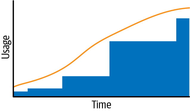
Figure 22-5. Commitment coverage when performed infrequently
Figure 22-6 shows a much more frequent commitment purchase program. The frequency isn’t always the same over time, but the resulting commitment coverage follows the resource usage growth tightly.
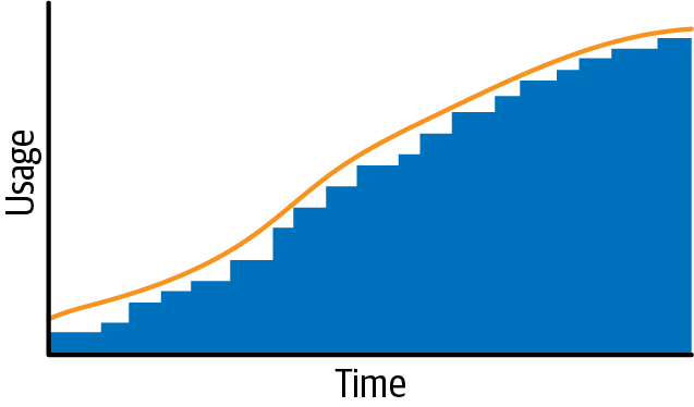
Figure 22-6. Commitment coverage when performed frequently
Schedule-driven cost optimization is fine to get started, but continuing to perform purchases slowly leaves savings on the table. However, looking at commitments too often will result in time wasted, so you need to strike a balance.
Tip
You can quickly determine when you’re missing your goals by using metrics with set targets.
Metrics will trigger alerts to perform optimizations only when needed. MDCO can be used for the entire gamut of available optimizations. It’s critical to measure metrics properly, so that optimizations are triggered at the right time. It’s also important to set achievable targets.
Setting Targets
For some metrics, like commitment coverage, we recommend setting a conservative goal at first and then working your way to a high target such as 80%. A low target does not make sense, however, for utilization. Applying a “start low” model to commitment utilization would end up costing you more than it saves.
Let’s look at applying metrics to usage reduction methods. Removing unused resources and resizing underutilized resources also generates savings. The total potential savings as a percentage of cost is referred to as a wastage percentage. A team spending $100,000 a month with potential savings of $5,000 would be said to have 5% wastage. Alternatively, a team spending $10,000 a month and a savings potential of $2,000 would have 20% wastage. Teams can be compared when measured this way, and generalized targets can be set for wastage. When wastage exceeds a set amount, you can focus on reducing it.
Taking Action
We mentioned that MDCO encompasses all three phases of the FinOps lifecycle. We’ve shown how you can use this data to build visibility, measure potential optimizations, and set goals based on these numbers, all of which are inform and optimize phase tasks, yet we’ve placed this chapter in the operate phase part of the book. That’s because the success of MDCO depends on what you do after you’ve set up reporting and alerting of MDCO and these alerts fire, requiring you to respond to needed changes in your optimization performance.
As previously mentioned, without clearly defined processes and workflows, it’s unlikely you’ll meet your organization’s FinOps goals. It’s important to specify who is responsible for actioning an MDCO alert, what the correct approval process is for things like buying new commitments, and what the correct order of operations is for modifying and/or exchanging existing commitments.
Have a preapproved commitment purchasing program within your organization. Giving the FinOps team the freedom to buy commitments as needed—up to a certain amount per month—reduces the lag time between a commitment coverage alert and the purchase of more commitments to cover the shortage. Improving processes helps reduce the delay in taking action.
Tip
There’s a fine balance between proactive and reactive. What should be reactive? What should be proactive? Don’t react to time as you would with cadence-driven cost optimization; aim to react to cost data as MDCO enables. Use this data to react faster. Capabilities like forecasting can help you predict when you will cross thresholds required before they happen, enabling you to be proactive. By ensuring this proactive data-driven prediction, you’ll be ready to react quickly to real-world cost scenarios that can have dramatic effects on your cloud bill.
Bring It All Together
MDCO gives you the confidence that metrics will trigger you to adapt when needed. It moves you from reacting to an arbitrary schedule on the calendar (such as monthly RI management) to reacting to changes in data. But don’t improvise your reaction; aim to have plans in place for the functional activities that you will do when the metric goes outside of the bounds, such as purchasing additional RI commitments. And be sure to plan for who will take which actions.
Ashley Hromatko, formerly Director of Cloud FinOps at Pearson, laid out this example—see Table 22-1—of how she used MDCO (coupled with assessment lenses from the FinOps Foundation’s Finops Assessment) to define a clear process for who would determine changes needed to a cost threat, and completed the loop with automation to action changes in the environment, which resulted in significant cost savings.
| Phase | Lens | Process | Action |
|---|---|---|---|
| Inform | Knowledge | Awareness of impact for change | 800+ AWS accounts and no lifecycle rule configured for S3 incomplete multipart uploads |
| Inform | Process | Who will make decisions | Spending 11K per month on incomplete multipart uploads, no single account is exceeding more than 1K |
| Optimize | Metrics | Baseline KPIs for success | FinOps submit policy to Cloud Governance board for review, vote to move to implement |
| Optimize | Adoption | How will implementation be communicated | Decision made for remediation after 14 days and ability to opt-out |
| Operate | Automation | Offload repetitive tasks to tooling | Cloud Custodian policy created by Cloud Management engineering team |
The outcome was a process that attached a lifecycle policy to all S3 buckets and automated the removal of incomplete multipart uploads after 14 days. The policy resulted in significant automated cost savings the next month, as shown in Figure 22-7.
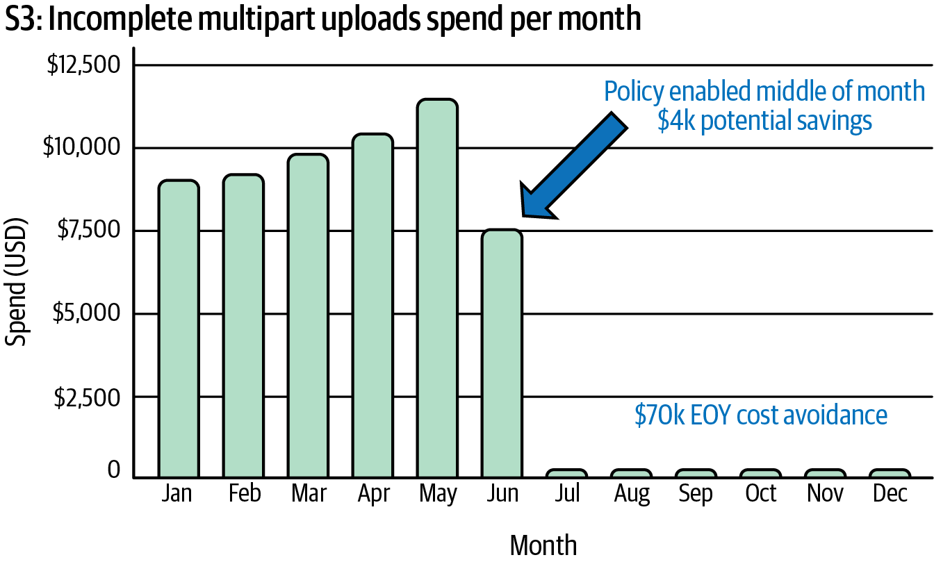
Figure 22-7. Spending decline after a multipart upload policy is put in place
Conclusion
Metric-driven cost optimization encompasses all three phases of the FinOps lifecycle, with visibility and targets driving the cost optimization process. Automation plays a major role in providing a repeatable and consistent process.
To summarize:
All cost optimizations are driven by metrics, and all metrics require achievable targets.
Computers should perform repeated data analytics and alert when metrics are off-target.
All changes being performed should be reflected in the metrics. Ultimately savings should increase, and cost optimization efficiency should remain high.
MDCO is about knowing exactly when is the optimal time to perform optimization processes.
Just when we believe we have this FinOps world under control, engineers innovate and introduce a whole new world on top of the cloud using containerization. Next, we look into the impacts of clusterization using containers and how you can use your existing FinOps knowledge to solve the new problems this creates.