
17
Comparison of Various Classification Models Using Machine Learning to Predict Mobile Phones Price Range
Chinu Singla1* and Chirag Jindal2
1 Department of Computer Science and Engineering, Punjabi University Patiala, Punjab, India
2 Department of Computer Science and Engineering, Thapar Institute of Engineering and Technology, Patiala, Punjab, India
Abstract
Classification is the Machine Learning technique used for classifying categorical data. In this chapter, different classification models are used to predict the price range of the different mobile phones based upon their features. The use and demand of Mobile phones seem to be at their peak today, and this trend does not seem to go down in the near future. Therefore, an efficient system needs to predict the mobile prices’ range based on its features. We have taken the mobile phone dataset containing information about their various features and functions for our research. After that, pre-processing is being performed to remove the ambiguities before applying the classification models. The Price range can be of any category between 0 and 3, where 0 represents cheapest and 3 costliest. We aim to find the classification model with the best results. Accuracy and R2 score are used to select the best model.
Keywords: Classification, mobile phones, decision tree, logistic regression, Naive Bayes, support vector machine KNN, accuracy, prediction
17.1 Introduction
Machine Learning (ML) is all about creating a machine that can be as close to the human mind as possible. The ML algorithms are created to copy the human approach of learning, which can sometimes be from previous knowledge like supervised learning or sometimes from new experiences like unsupervised learning [1]. Since price is the most essential and foremost factor that comes into a person’s mind when anyone thinks about buying or exploring something, one has to keep it as an output variable. Budget is the main thing that decides what a person is looking for. Our model will help the customer in finding the features and phones available in his budget.
The application of Artificial Intelligence is possible through Machine Learning Techniques, which are mainly regression and classification. Classification is used to analyses discrete data types, while regression is used for continuous data types [2]. Here output variable is in the form of discrete data, so we apply various classification models. Also, this is an example of supervised learning since the previous values of the data are already known [3]. For our application, code is written in Python and the four main libraries used are numpy, pandas, matplotlib, and scikit learn [4]. Different classification models mentioned here are Logistic Regression, KNN, SVM, Decision tree, and Gaussian Naive Bayes. We apply a few opti-mization techniques to our dataset, such as feature scaling [5].
Mobile phones are the most in-demand and must device in today’s world. Everyone has one and is planning to update it. There is a somewhat race going on between different companies who come up with a better mobile phone. In this case, people require a system that can help them choose the phones in their budget and the features they require [6]. Keeping this rising trend of mobile phones in our mind, we take the dataset of the mobile phones and the features they possess. Like mobile phones, our research can be applied to laptops, cars, and other gadgets, just with a few minor changes. The dataset contains many mobile phone features like battery, camera, RAM, memory, etc., and based upon these features, we can predict price ranges.
Here, we predict the price of these mobile phones based upon the features which they have. We have implemented five classification models in total and tried to draw a comparison between these models based upon their accuracy and R2 score.
The organization of the research papers as follows. Under section 17.2, explanation of dataset and classification techniques, followed by data pre-processing in section 17.3 and the application of these classification models in a further section. In the end, metrics and finding the most suitable model are applied and elaborated under Section 17.6. Lastly, the conclusion and future scope are elaborated in Section 17.7.
17.2 Materials and Methods
17.2.1 Dataset
In this chapter, the data we consider is the “Mobile Price Classification” training and testing dataset from Kaggle [7]. The dataset contains the features of Mobile Phones along with their Prices [7].
There are 21 features in the dataset, with the 21st representing the price, as shown in Table 17.1. Some of the features are discrete data, while some are continuous data(Mobile Weight). The ones in the form of discrete are further of two types, i.e., binary (Bluetooth and Wi-Fi) and Multi-valued (Camera Pixels).
17.2.2 Decision Tree
A decision tree is one of the influential and most suitable classification algorithms used in Machine Learning. The concept behind it is that it causes the best possible split of the tree based on our features. It can be made in two ways: Entropy and Gini Index. Here, we have used Gini Index. The results remain the same in both cases [8].
It is a powerful method not just for classification and prediction of data but also for interpretation and data manipulation. Decision tree is also robust to outliers and provides an easy way of handling missing values.
Table 17.1 Some of the dataset values.
| Battery | BT | Clock speed | Dual SIM | Int memory | Depth | Width | N_cores | pc | RAM |
|---|---|---|---|---|---|---|---|---|---|
| 842 | 0 | 2.2 | 0 | 7 | 0.6 | 188 | 2 | 2 | 2549 |
| 1021 | 1 | 0.5 | 1 | 53 | 0.7 | 136 | 3 | 6 | 2631 |
| 563 | 1 | 0.5 | 1 | 41 | 0.9 | 145 | 5 | 6 | 2603 |
| 615 | 1 | 2.5 | 0 | 10 | 0.8 | 131 | 6 | 9 | 2769 |
| 1821 | 1 | 1.2 | 0 | 44 | 0.6 | 141 | 2 | 14 | 1411 |
| 1859 | 0 | 0.5 | 1 | 22 | 0.7 | 164 | 1 | 7 | 1067 |
| 1821 | 0 | 1.7 | 0 | 10 | 0.8 | 139 | 8 | 10 | 3220 |
Decision Tree has a disadvantage as well that it can subject to under- fitting and over fitting especially when the dataset is small. Strong correlation between input variables of the decision tree can be another problem for us as those variables are selected sometimes which just improve model statistics and the outcome of interest is actually not related to them. Skewed data can be handled by decision tree without the need of transformation.
Gini Index computes how often a randomly selected value would be wrongly recognized. This means the attribute with less Gini Index should be preferred. Gini Impurity can be calculated with the help of the formula shown in Eq. (17.1):
Where h is the probability of belonging to the current attribute and n is the no. of attributes.
17.2.2.1 Basic Algorithm
We import the DecisionTreeClassifier from sklearn.tree library. The code for decision tree is as follows:
- From sklearn.tree import DecisionTreeClassifier
- classifier= DecisionTreeClassifier(criterion=’entropy’, random_state=0)
- classifier.fit(x_train, y_train)
Here, two main parameters are considered;
“criterion=’entropy’: It measures quality of split.
random_state=0”: To generate same random numbers.
17.2.3 Gaussian Naive Bayes (GNB)
GNB is an algorithm works on the basis of Bayes theorem. In Gaussian Naïve Bayes, sequential values linked with each characteristic are supposed to be distributed in accordance to the Gaussian distribution. It has a principle that every pair of classified features is independent of each other [9].
In this, continuous values of each feature follow Gaussian distribution. It produces a bell-shaped curve that is symmetric about the mean of the feature values.
Naive Bayes is very fast and works quite well in real life based problems. Naive Bayes can be of further types as well:
Multinomial Naive Bayes: The frequency with which specific events were created by a multinomial distribution is expressed by feature vectors. This is the most common event model for document categorization.
Bernoulli Naive Bayes: Features are independent Booleans that describe inputs in the multivariate Bernoulli event model. This model, like the multinomial model, is useful for document classification tasks when binary term occurrence characteristics instead of term frequencies are used.
Bayes theorem finds the probability of an event occurring given another event that has already occurred. Bayes theorem formula is given by (Eq. 17.2):
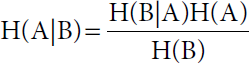
Where H (A) is the probability of A, H (B) is the probability of B, and H (B|A) is the probability of event B given that event A has already occurred [10].
This formula gives the probability of happening of event A given that event B has already happened.
17.2.3.1 Basic Algorithm
We used the Naive Bayes classifier to the Training dataset. The code for the same is as follows:
- from sklearn.naive_bayes import GaussianNaiveBayes
- classifier = GaussianNaiveBayes()
- classifier.fit(a_train, b_train)
17.2.4 Support Vector Machine
SVM works for both classifications and regression issues. The objective of SVM is to build the boundary of decision which can separate multidimensional coordinates to classes so that one can quickly use the latest data set to the category it belongs to. SVM chooses the extreme point that helps create the hyper-plane [11], as shown in Figure 17.1. These extreme endpoints are called support vectors and give the algorithm its names [12]. SVM can also be made nonlinear using different types of kernel. Among many kernels, one of the most common is anisotropic radial basis. Therefore it can produce accurate results even when the data is nonlinear and cannot be separated by a single line of plane.
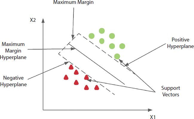
Figure 17.1 Two different classes using SVM.
The figure above shows how SVM draws a fine line which is equidistant from both the categories with the help of Positive, Negative Hyperplanes, and Maximum Margin.
17.2.4.1 Basic Algorithm
SVM is implemented using the following code: We extract support vector class from Sklearn.svm library. The code is as follows:
- from sklearn.svm import SVC
- classifier = supportvector(kernel=’linear’, randomstate=0)
- classifier.fit(a_train, b_train)
Since data is linearly separable, we’ll use the linear kernel. Afterwards we used the classifier to the training dataset(a_train, b_train).
17.2.5 Logistic Regression (LR)
LR is mainly used for binary outcomes but can also be used for non-binary outcomes. It is named after the function it is based on, i.e., Logistic function, also known as Sigmoid Function. It is an S-shaped Curve that can take any real-valued number and map it into a value between 0 and 1 but never strictly at the boundaries as depicted in Figure 17.2.
It becomes a classification technique only when a decision threshold is applied based upon the classification problem [13]. This technique is of further three types.
- Binary Logistic Regression: This is used when output is binary or has only two possible outcomes. For example 0 or 1.
- Multinomial Logistic Regression: This is the one we used here. This is used when output variable has three or more possible values without ordering as in our case.
- Ordinal Logistic Regression: This is used when output variable has three or more possible values with ordering.
17.2.5.1 Basic Algorithm
We create a classifier for implementing Logistic Regression as given below:
- from sklearn.linear_model import LogisticRegression
- classifier= LogisticRegression(random_state=0)
- classifier.fit(x_train, y_train)

Figure 17.2 Logistic regression curve and its equation.
17.2.6 K-Nearest Neighbor
KNN is a classification algorithm in which the data point is assigned the category most of its neighbors belong to. KNN assumes that things which are closer to each have similar behavior. Apart from Classification, KNN can also be used for search and regression. No need to create a model, tweak a few parameters, or make any more assumptions in KNN. The fundamental downside of KNN is that it becomes substantially slower as the volume of data grows, making it an unsuitable solution in situations when predictions must be made quickly. In the case of classification and regression, we observed that the best way to choose the proper K for our data is to try a few different Ks and see which one performs best.
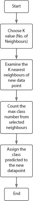
Figure 17.3 KNN implementation steps.
First, we select the number k, usually the square root of n, i.e., the total number of data points. Then we sort all data points based upon their Euclidean distance from the given data point as shown in Figure 17.3. Euclidean distance is calculated by using Eq. 17.3:
Where r1 and s1 are the coordinates of the given data point in focus and r2 and s2 are the coordinates of the data point from which we calculate distance. Then we select the first K data points and check their class. Our data-point is assigned the class to which the majority of those K data-points belong [14].
17.2.6.1 Basic Algorithm
We fit the K-NN classifier to the training data. We first import the KNeighborsClassifier class of Sklearn Neighbors library. After that, we create the Classifier object of the class. The Parameter of this class will be n_neighbors: The number of neighbors to be considered.
- metric=’minkowski’: Parameter for deciding distance between two objects.
- p=2: It is equivalent to the standard Euclidean metric.
The code is as follows:
- from sklearn.neighbors import KNeighborsClassifier
- classifier= KNeighborsClassifier(n_neighbors=5, metric=’ minkowski’, p=2 )
- classifier.fit(x_train, y_train)
17.2.7 Evaluation Metrics
The Accuracy, R-score, and confusion matrix are being used to evaluate the models described previously.
A confusion matrix is an N × N matrix that summarizes the Accuracy of the Classification Model’s predictions. N is the number of classes. Here N = 4. In binary problem, N = 2. Confusion Matrix is a correlation between the actual labels and the models’ predicted values. One axis represents actual values while the other represents predicted values [15].
Accuracy is the total number of values accurately analyzed upon the total number of values predicted by the model. The formula for Accuracy is given by Equation (17.4):

True Positives means the accurate values predicted by the model, and True Negative means, the negative values analyzed by the model. All Samples are the total number of values predicted.
17.3 Application of the Model
In the study, five models are used independently to predict the class of the mobile phone price, as shown in Figure 17.4. First, we read the dataset and assign the input and output variables to x and y, respectively.
Firstly we split the dataset into training and testing with a ratio of 3:1, and our model will be trained on 75% dataset while the rest of the 25% dataset will be used to test the model. After that, we performed feature scaling on the dataset to narrow the range of the values. A technique we use here is standardization [16]. The whole procedure to predict the prices of mobile phones is illustrated in Figure 17.4.
The feature scaling was followed by the actual implementation of the classification models whose detailed implementation is explained below. Once the models were implemented, we evaluated the results of the same using metrics library. At the end, these results were compared and we found out the best and the worst in this chapter.
Figure 17.5 roughly divides our chapter into four rough categories of data collection, data preprocessing and model creation, model optimization and evaluation and finally model deployment. It shows further the sub steps of each step.

Figure 17.4 Implementation steps.

Figure 17.5 Flowchart to predict mobile phone price range.
17.3.1 Decision Tree (DT)
Here we implement a decision tree here using the criterion entropy and keeping the random state = 0 so that every time we run the code [17], the same values are chosen. After implementing the decision tree, we get the confusion matrix (Figure 17.6) where rows shows the predicted values while column shows the actual values.
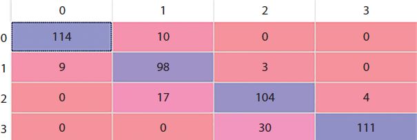
Figure 17.6 Decision tree confusion matrix.
17.3.2 Gaussian Naive Bayes
We use sklearn to import and implement Gaussian naive Bayes. There is no need for parameters while implementing the Naive Bayes.
The confusion matrix (Figure 17.7) where rows shows the predicted values while column shows the actual values we get is.
17.3.3 Support Vector Machine
Firstly we import SVC from sklearn. While implementing SVM, we require an input parameter called Kernel. In this case, we take Kernel as linear.
The resultant confusion matrix (Figure 17.8) where rows shows the predicted values while column shows the actual values is.
17.3.4 Logistic Regression
We import Logistic Regression from sklearn.linear_model and give the random state as the only input parameter as similar to decision tree. The confusion matrix (Figure 17.9) where rows shows the predicted values while column shows the actual values is as follow.
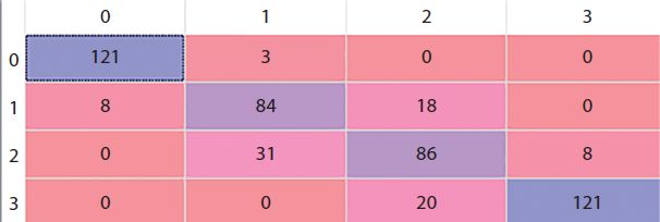
Figure 17.7 Gaussian Naive Bayes confusion matrix.
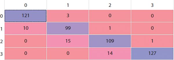
Figure 17.8 Support vector machine confusion matrix.
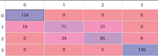
Figure 17.9 Logistic regression confusion matrix.
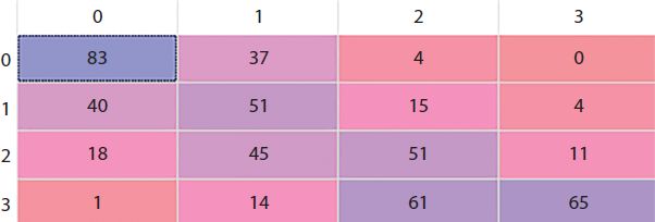
Figure 17.10 KNN confusion matrix.
17.3.5 K Nearest Neighbor
K neighbors classifier is imported from sklearn. Neighbors to implement KNN. The parameters required are n_neighbors, metric, and p-value. The n_neighbors is the k value we use in our model building. The distance Metric we use is Minkowski, whose formula is.
Where u and v are the coordinates of the data point in focus.
The third parameter is the p-value in the above formula, which is 2 in the case of Euclidean Distance which we use for our model [18]. The confusion matrix (Figure 17.10) where rows shows the predicted values while column shows the actual values.
17.4 Results and Comparison
We calculate R2 as well as the Accuracy score for all the five models we applied. The Accuracy for all the models turned out to be pretty good except for the KNN. The Accuracy score for Decision Tree, Naive Bayes, SVM, and Logistic Regression turns out to be in a pretty close range that is 85.4%, 82.4%, 91.2% and 83.2%, respectively.
The accuracy of K Nearest Neighbor turned out to be just 50% since we took the number of neighbors k as a fixed number instead of using the generic rule of root n where n is the total number of data points. The Bar plot (Figure 17.11) given below compares the accuracy scores of the different models. Here the model of Decision Tree, Naive Bayes, Support Vector Machine, Logistic Regression, and K Nearest Neighbor are written in the form of DT, NB, SVM, LR, and KNN respectively. The Bar plot shows how the accuracy of SVM is the highest while that of KNN is the lowest thereby giving us a clear idea of the chapter.
We also calculate the R2 score or coefficient of determination for all the models. It came out to be 0.888, 0.865, 0.933, 0.871, and 0.421 for Decision Tree, Naive Bayes, SVM, Logistic Regression, and KNN. The same trend is observed in the case of R2 score as well since the score of KNN is way less than that of others which are in a pretty close range to each other. The Bar Plot (Figure 17.12) showing the R2 scores of different classification Models. Here the model of Decision Tree, Naive Bayes, Support Vector Machine, Logistic Regression, and K Nearest Neighbor are written in the form of DT, NB, SVM, LR, and KNN respectively. The Bar plot shows how the R2 score of SVM is the highest while that of KNN is the lowest thereby giving us a clear idea of the chapter.
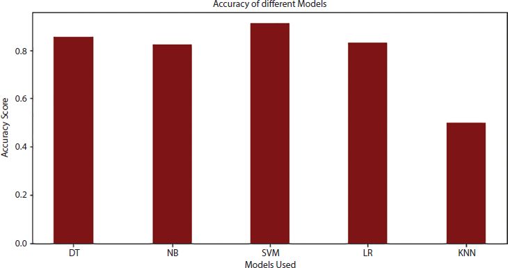
Figure 17.11 Accuracy of different models.

Figure 17.12 R2 score of different model.
The similar nature of the above two plots also shows us that the accuracy and R2 score vary according to each other and are somehow codependent thereby confirming a directly proportional relationship between them. As we can see that the model which have the highest accuracy also displays highest R2 score i.e. SVM in this case while the model giving the lowest accuracy also gives the lowest R2 score i.e. KNN in this case. The relationship between the Accuracy and R2 score can be displayed by the following formula:
Where K is a constant.
Table 17.2 describes comparison of different machine learning models in terms of accuracy and R2 score.
The above table summarizes the entire comparison between the five models for us. It compares the five models in six different contexts. Basic Concept tells us the algorithm or the basic principle the model is based on. Then number of parameters tells the number of parameters that are required in the implementation of each model which is maximum in the case of K Nearest Neighbor, i.e., 3 while 0 in Support Vector Machine which is then followed by the name of those parameters. The next two contexts are the Accuracy and R2 score calculated by us as shown above. The last context tells us their limitations or what these models lack in.
Table 17.2 Comparison of various machine learning models.
| Features | Decision tree | Naive bayes | Support vector machine | Logistic regression | K-nearest neighbors |
|---|---|---|---|---|---|
| Basic concept | Based on Entropy or information gain | Based on Bayes Theorem | Based on extreme point boundary Based differentiation | Based on application of Sigmoid function on Linear Regression | Based upon K Closest neighbors |
| Number of parameters | 2 | 0 | 1 | 1 | 3 |
| Parameter names | Criterion and random state | Kernel | Random State | Number of neighbors, metric and p value | |
| Accuracy | 85.4% | 82.4% | 91.2% | 83.2% | 50% |
| R2 score | 0.888 | 0.865 | 0.933 | 0.871 | 0.421 |
| Limitations | Unstable as a little change in the dataset can cause massive change in the tree structure. | If it encounters a case or category which was not present in the training dataset, it will assign it 0 automatically | It does not perform very efficiently if the dataset has noise. | It always assume linear relationship between dependent and independent variables. | Gets effected by the amount of data and irrelevant features. |
17.5 Conclusion and Future Scope
In the study, we compared the five different classification models on the dataset of mobile phones, taking the price class as the output variable. We split our data into training and testing datasets and performed feature scaling as well. Then we applied the classification models. We find their Accuracy Score and R2 score, and based upon the values of these scores, we discovered that the Support Vector Machine proves to be the suitable model in this case with the Accuracy of 91.2% R2 score of 0.933. We also found that all the models except for KNN showed decent results and concluded that the low value of K taken compared to the size of the dataset is the reason behind the poor performance of KNN. The results of Decision Tree, Logistic Regression, and Naive Bayes are pretty close.
Further improvement can be made by applying a combination of multiple classification models or changing some parameters of the already applied models. Random Forest can also be applied to the dataset. Few more steps can be included in the pre-processing part to make the dataset consistent and even better.
References
- 1. Talwar, A., and Kumar, Y. Machine Learning: An artificial intelligence methodology. Int. J.of Eng. & Comput. Sci., 2, 12, 3400–3404, 2013.
- 2. Singh, A., Thakur, N., S., A., A review of supervised machine learning algorithms. D. (INDIACom), 2016, ieeexplore.ieee.org.
- 3. Singh, A., Thakur, N., and Sharma, A. A review of supervised machine learning algorithms. In 2016 3rd International Conference on Computing for Sustainable Global Development (INDIACom), 1310-1315, IEEE, 2016, March.
- 4. Albanese, D., Merlere, S., Jurman, G., Visintainer, R., MLPy: High-performance python package for predictive modeling. NIPS, MLOSS Work, 2008.
- 5. Akritidis, L. and B., P., A supervised machine learning classification algorithm for research articles. P. of the 28th A. A. Symposium, 2013, pp. 115–120, 2019, doi: 10.1145/2480362.2480388, dl.acm.org.
- 6. Arroyo-Cañada, F.-J., Lafuente, G., J., Influence Factors in Adopting the m-Commerce Resources, and Users, pp. 46–50, 2011.
- 7. Mobile price classification | Kaggle, 2018. https://www.kaggle.com/iabhishek official/mobile-price-classification.
- 8. Song, Y. Y., and Ying, L. U. Decision tree methods: Applications for classifi-cation and prediction. Shanghai archives of psychiatry, 27, 2, 130, 2015.
- 9. R.-I., I., An empirical study of the Naive Bayes classifier. 2001 Workshop on Empirical Methods in Artificial and Undefined, 2001, cc.gatech.edu.
- 10. Friedman, N., Geiger, D., Goldszmidt, M., Bayesian network classifiers. Mach. Learn., 29, 2–3, 131–163, 1997.
- 11. Cortes, C. and V., V., Support-vector networks. Mach. Learn., Springer, 20, 273–297, 1995.
- 12. Evgeniou, T. and Pontil, M., Support vector machines: Theory and applications. Lect. Notes Comput. Sci., 2049 LNAI, 249–257, 2001.
- 13. Peng, C., Lee, K., I., G., An introduction to logistic regression analysis and reporting. J. Educ. Taylor Fr., 96, 1, 3–14, 2002, doi: 10.1080/00220670209598786.
- 14. Wang, L. Research and implementation of machine learning classifier based on KNN. In IOP Conference Series: Materials Science and Engineering, 677, 5, 052038. IOP Publishing, 2019 December.
- 15. Moksony, F., and Heged, R. Small is beautiful. The use and interpretation of R2 in social research. Szociológiai Szemle, Special issue, 130–138, 1990
- 16. Nasser, I., Al-Shawwa, M., Abu-Naser, S., Developing artificial neural network for predicting mobile phone price range. Int. J. Acad. Inf. Syst. Res., 3, 1–6, 2019.
- 17. Han, L.W., Manipulating machine learning results with random state, Towards Data Science, 2019, https://towardsdatascience.com/manipulating-machine-learning-results-with-random-state-2a6f49b31081.
- 18. Güvenç, E., Cetin, G., K., H., Comparison of KNN and DNN classifiers performance in predicting mobile phone price ranges. Adv. Artif. Intell., 1, 1, 19–28, 2021, dergipark.org.tr.
Note
- * Corresponding author: [email protected]