
Chapter 4. Fundamental Detector Types
As we will often note, there are four flavors or types of data:
- Images → imaging
- Brightness → photometry
- Color → spectroscopy
- Timing → variability
Each involves a separate data goal, and together all four fold into your detector profile and its bandwidth needs (Example 4-1).
Brightness: e.g. 3.846 x 1,026 W in luminosity, 4.83 absolute magnitude

Spectral: e.g. "color image plus IR/thermal"

Timing: e.g. "On during the day, off at night"
You can also mix these data goals. An imaging spectrometer is a camera (imaging) that gives you a separate data frame for each color. Instead of seeing one picture, you can compare, for example, the image in red against the image in blue.
A light curve is how the imaging, brightness, or color of an object changes over time. Light curves are crucial for analyzing the variability of a changing object. Light curves are often used to find asteroids or even extra-solar planets through occultation (one object moving in front of another). A brightness shift often indicates occultation.
A spectral change can indicate an object in motion, through the Doppler Shift. A light curve of spectra + timing can provide information on occultation as well.
If you put together any pair of the Image/Brightness/Spectra/Timing elements, you get a new data item to track. Consider these combinations:
- position + timing = movement
- brightness + timing = variability
- color + timing = change in composition or temp
- position + brightness = magnitude
- position + color = what and where
- brightness + color = more composition info
The Eternal Fight: Resolution Versus Brightness
You can capture something bright, or you can subdivide it to get more information, but you can’t capture all the information in all possible ways.
The modern conflict is data bandwidth versus data accumulation. We are always starving for photons, either because the source is dim, or our detector is small or inefficient, or our download bandwidth is limited—no matter what, you can’t get as many photons as you want.
We call this being photon limited, literally without enough photons to see the object. Most astronomical observations by the Hubble Space Telescope, for example, are photon limited because the objects themselves are very distant and thus faint.
We also describe being bandwidth limited: not able to deliver enough data. The object may be quite visible, but (like a slow internet connection) you simply can’t access it. The STEREO mission, which uses two satellites with 11 instruments to stare at the Sun, is an example where there are certainly enough photons available, but we lack enough communications bandwidth to transmit the multiple Terabytes needed to Earth.
Active Detectors
So far, we have focused on traditional passive detectors. A source emits or reflects light, which the sensor captures. Active detectors provide their own light (or other) source. For example, a bat’s sonar works because the bat emits a high pitched sound, then listens to its reflected echo to determine its position. It’s a pity sound doesn’t travel in space, or we could try this on a satellite.
Instead, Radar and LIDAR send out a beam of light (radio waves for Radar, laser pulses for LIDAR) then capture the return bounce and analyze how long that light took and how it changed to determine what is there. You could use a light source as a flash to either illuminate a target, or as a probe for a detector on the other side that looks at how the light was changed.
Active detectors, however, typically consume far more power than a passive detector, not the least because they need a passive detector element plus the addition of the active source. For picosatellites, use of active detectors is very cutting edge. Fortunately, in terms of interface, bandwidth calculation, and all the other work in this book, the same sensor theory applies. You may be setting yourself up with a more complex problem by building an active detector, but the principles remain sound.
Tradeoffs
Let’s look at image brightness. Do you want a bright image with low detail, or very fine detail but a dim image? A high image resolution or a brighter image? Color information or a brighter image? Quick variability or a brighter image?
For timing accuracy, we consider both how long it takes to capture data, and how long it takes to prepare for the next frame. These are called integration time and cadence, respectively.
- Integration time, a.k.a. shutter speed
- How long you have to stare to acquire the image
- Cadence
- How quickly you can take successive images (due to readout time, processing time, etc.).
Both lead to your limits in timing accuracy. A sample timing accuracy calculation is: if it takes 3 seconds to acquire an image, your best time resolution is +/– 3 sec. If you can only take one image every minute, your best time resolution is +/– 60 sec.
The effects of timing issues include smearing—the source moved or changed during the exposure—and gaps—the source moved or changed in between frames (while you weren’t looking).
There’s a direct analogy to handheld digital cameras. Depending on the light level, you may or may not be able to see your target. There’s a lag in between frames. If you want to pursue sports photography, you need a fast shutter speed and lots of light. Looking at detector tradeoffs involves a key set of decisions you need to examine before you shop around for a sensor. The issues to discuss are whether it is imaging or takes a single value, how many colors it can see, how accurately it can discern different brightness levels, and how quickly and how often it takes data. We’ll work on these four—Imaging, Spectral, Brightness, and Timing—but first, we need to examine the sizes and framing of the actual targets we wish to examine. For that, we’ll discuss Field of View.
Imaging Detectors
Detectors are specified with a given Field of View, which is the angular size they view in units of degrees (or the smaller increments of degrees: there are 60 arcminutes in 1 degree, and 60 arcseconds in 1 arcminute). A wide, panoramic field of view might be 180 degrees; a narrow zoom-in might be a degree or less. This is identical to the wide/zoom button on any digital camera.
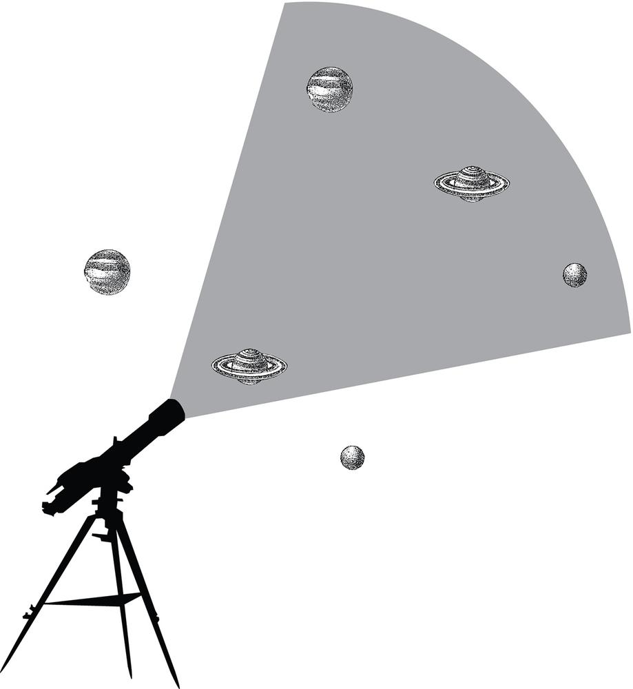
Mapping Coverage to Pixels
In Figure 4-1, we show a sample FOV of about 25 degrees. At close range, we can only see 1 of the 3 objects, but it fills the whole field of view, so we’ll get a nice big image of it. At a longer range, we can see all 3 of the 3 objects, but each one only fills a third of the field of view, so their size in the image (and thus their resolution) will be smaller.
For astrophysical missions, this angular field of view is all we need. For Earth observing and planetary and military sensing, however, we need to figure out how this angular measure maps to a Ground Field of View (GFOV)—how much area of the ground (in square kilometers or square miles) our detector will see.
To convert from angular FOV to ground FOV, you use simple trigonometry. If you are looking straight down, your FOV is basically a large isosceles triangle, where the ground is the base and your angular FOV is your top triangle angle. Using triangle math, the result is that the GFOV * 2 * (height_above_ground) = tan(angular_FOV/2).
For Earth Observing (EOS) maps, then, we can talk about our FOV in terms of area, of rectangular shapes. The calculation for “my image, map, scene that I’m capturing” to “detector elements” uses just multiplication to figure out our units:
Physical area/number of pixels = pixel size
or, assuming some physical area in units of kilometers (km):
Length_km/x_pixels by Width_km/y_pixels = (# of x pixels) by (# of y pixels)
Phrased another way, an A x B km physical area mapped onto an i x j detector means each pixel covers (A/i) km x (B/j) km, as shown in these mappings:
Case 1: Square area, square detector
    Covering an area 100 x 100 km using:
        a 10 x 10 pixel array:    1 pixel = 10 km x 10km
        a 100 x 100 pixel array:  1 pixel =    1km x   1km

Case 2: Rectangular area, square detector
    Covering an area 20 x 100 km using:
        a 10 x 10 pixel array:    1 pixel =   2 km    x 10km
        a 100 x 100 pixel array:  1 pixel =   0.2km  x  1km

Case 3: Square area, Rectangular detector
    Covering an area 100 x 100 km using:
        a 20 x 10 pixel array:    1 pixel =  50 km  x 10km
        a 200 x 100 pixel array:  1 pixel =  0.5 km x   1km
Bear in mind we are assuming a straight downward (nadir) pointing. If you tilt your detector—as with the image of TRMM shown in Figure 4-2—your footprint calculation becomes more complex. However, the basic math does not change: deduce the geometry, figure out your footprint area, and divide by the number of pixels available.

Sampling and Bandwidth Calculations
Most picosatellites are going to be bandwidth-limited rather than photon-limited. Photon-limited means you are looking at a faint source, such as astronomical objects. Bandwidth-limited, in contrast, means your sensors can get more data than you can transmit to the ground.
There are four factors that affect how much bandwidth you use:
Imaging (I): Are you taking an image (A by B pixels, requiring A*B data points), or are you just taking a single value like a temperature, an electric field strength, a magnetic field strength, or other single data point? Landsat-7’s ETM camera is actually a scanner that takes a narrow 1-D line swath view and then (like a photocopier) combines subsequent lines into 2-D images. Typical Landsat-7 “scenes” might be 238×243 pixels. High definition video often uses 1,280×720 pixel images or larger.
(Landsat-7 covers the entire Earth with 57,784 scenes every 16 days: each scene is 233×248 pixels. That works out to roughly one scene taken each second. Because it takes scans and ends up covering the full Earth, you can really chop up its data any way you wish.)
Once we have a chosen detector size (our imaging resolution), we can figure out the bandwidth needed for our given quartet of resolutions (imaging, photometric, spectral, and timing).
Spectral or Colors (S): The number of colors or spectral bands you capture will multiply your bandwidth needs. If you take a single band, akin to monochrome images, there is no multiplier. However, if you wish to sample several bands (also called colors or channels), that will cost you. A color image, for example, requires three times the storage of a black and white (B&W) image: one data point each for the red, green, and blue elements that make up the full color.
If you are sensing past optical, you can sample discrete bands by providing filters that let you chop up a monochromatic range (such as IR) into bands. For example, the Landsat-7 optical plus infrared camera splits up the range of IR into 7 bands that include not just our ordinary 3 bands of red/blue/green color, but the near-IR (0.76–0.90 um), mid-IR (1.55–1.75 um and 2.08–2.35 um), and thermal IR (10.40–12.50 um). This gives more information, but also means they must transmit seven times the amount of data relative to just sending a B&W image.
Brightness levels (B): The accuracy of your detector in terms of number of bits of data used to map brightness sets your basic data unit.
If you need to store a number between 0 and 255, you have 256 distinct values. 28 is 256, so you can use that calculation to determine that you need 8 bits to store a value between 0 and 255. Similarly, if you need to store a value between 0 and 1,023, you’ll need 10 bits of storage because 210 is 1,024.
These numbers correspond to how well you can discern the contrast in a scene or element. If you are providing a coarse 8 different levels of brightness (equivalent to 8 different crayons to cover from all white to all black), you are using 23 data values, or 3 bits. If you want finer shading, say 64 levels, that is 26 data values and thus 7 bits. Landsat-7 uses 8-bit data (0–256) for its images. High-def video may be 12-bit data or higher.
Here are some common bit and byte measurements:
| Data Size | Abbreviation |
8 bits | 1 byte |
103 bytes | 1 kilobyte |
106 bytes | 1 megabyte |
109 bytes | 1 gigabyte |
Timing (T): One key element of a detector is how often you wish to sample it get to get data. If you take one data sample (one frame, one temperature measurement, etc.) per day, that’s probably a safe, low bandwidth situation. If you instead need to send down high-definition video at 32 frames per second, that’s going to be high bandwidth.
It can be weird to think of, for example, a thermometer as a 1-pixel detector. You could rename Imaging to Elements if you wish. A thermometer is a 1-element detector; a 128–128 camera is a 128*128 element detector.
Our bandwidth calculation is pretty easy, as you just multiply these items to get a total, often converting from native bits into bytes (1 byte = 8 bits) and kilobytes (103 bytes), megabytes (106 bytes), gigabytes (109 bytes) or terabytes (1012 bytes).
You can determine the bandwidth your satellite needs with this equation:
Bandwidth = Image_size * Number_of_colors * Bits_per_pixel * Data_rate
(* 1 byte/8 bits)
Or, put another way:
Bandwidth = Imaging Res * Spectral Res * Photometric Res * Timing Res
(* 1 byte/8 bits)
So let’s look at three detectors of wildly varying type.
Temperature sensor, measures once/minute, uses 8 bits to encode number:
Bandwidth = 1 temperature * 1 band * 8 bits * 1/minute = 8 bits per minute, or 1 byte per minute.
Landsat-7 233×248 scene, 8 bands, 8-bit data, one taken per second:
Bandwidth = 233 * 248 * 8 * 8 bits * 60/min = 27.7 Megabytes per minute.
High-def streaming video at 1280×720, color (3 bands), 12-bit data, 32 frames per second:
Bandwidth = 1,280 * 720 * 3 * 12 * (32*60) = 8 Gigabytes per minute!
Here’s another sample scenario, a very plausible one you might fly. Assume a CubeSat with low resolution B&W images once per hour:
| Measuring | Resolution |
Imaging | 32×32 pixels |
Spectral | Grayscale → 1 channel |
Brightness | 256 brightness levels (8 bits/pixel) |
Timing | 1 frame each hour = 24/day |
For this low-resolution CubeSat case, our data size = 32 * 32 * 1 * 8 * 24 * 1 byte/8bits = 24,576 bytes = 24 KB per day!
If we downloaded this at the typical packet radio speed of 9,600 bps (a.k.a. 1,200 bytes/sec, a.k.a. 1.2 KB/sec), we need only a 17 second downlink.
Here’s another sample, an EOS satellite with medium-high resolution color images every minute:
| Measuring | Resolution |
Imaging | 1024×1024 pixels |
Spectral | color RGB → 3 channels |
Brightness | 1024 brightness levels (10 bits/pixel) |
Timing | 1 frame each minute = 1440/day |
For this medium resolution case, we require more bandwidth as we are gathering more data. Our data size = 1,024 * 1,024 * 3 * 10 * 1,440 * 1 byte/8bits = 5.6×109 bytes =~ 6 GB per day!
You can see why picosats are often used for in situ measurements of the local space environment: temperature, fields, brightness, images, and fast data rates will balloon your bandwidth needs.
Fully understanding a sensor involves all four aspects—Imaging, Brightness levels, Spectral levels, and your timing. Each has synonyms: imaging can also be number of detector elements, particularly for non-picture sensors. Brightness can be called photometry, and photometric brightness is a synonym for “how bright light is.” In contrast, you can also talk about temperature brightness or just about any variable and how strong its signal is. So you can think of brightness as signal strength and ability to sense contrast. A bit wordy, but it’ll do.
And, of course, we talk about Spectral or color choices, which can also be called bands or channels—particularly if you are going past visible light to the longer wavelengths of IR, submillimeter, microwave, and radio; or the shorter wavelengths of UV, X-ray, or gamma ray.
This synonym soup of multiple terms arises primarily because different scientists and engineers working in different fields all have their own particular form of jargon. Only in the past few decades has there been more combined multi-instrument work, resulting in the need to learn many synonyms.
Timing is often timing, timing resolution, capture speed, shutter speed, cadence (time between observations), revisit time (time before you return to the same spot), and a myriad of other terms. In this case, each term has a very specific meaning, but they all work together to define how quickly and how often you measure your targets. Table 4-1 summarizes each category and what it lets you determine about your target.