8
Two Qubits, Three
Not only is the Universe stranger than we think,
it is stranger than we can think.
In the previous chapter we defined qubits and saw what we could do with just one of them. Things now start to get exponential with every additional qubit added, because entanglement allows the size of the working state space to double.
This chapter is about seeing how multiple qubits can behave together and then building a collection of tools to manipulate those qubits. These include the concept of entanglement, which is a requirement to do quantum computing. We also examine important 2-qubit gates like CNOT and SWAP. This will lead us into chapter 9 and chapter 10 where we look at algorithms and build circuits that use this machinery.
All vector spaces considered in this chapter are over C, the field of complex numbers introduced in section 3.9 . All bases are orthonormal unless otherwise specified.
Topics covered in this chapter
8.2 Entanglement
8.2.1 Moving from one to two qubits
8.2.2 The general case
8.2.3 The density matrix again
8.3 Multi-qubit gates
8.3.1 The quantum H⊗n gate
8.3.2 The quantum SWAP gate
8.3.3 The quantum CNOT / CX gate
8.3.4 The quantum CY and CZ gates
8.3.5 The quantum CRϕz gate
8.3.6 The quantum Toffoli CCNOT gate
8.3.7 The quantum Fredkin CSWAP gate
8.4 Summary
8.1 Tensor products
In this section I introduce the linear algebra construction of a tensor product. If the direct sum seems to concatenate two vector spaces, then the tensor product interleaves them. In the first case, if we start with dimensions n and m, we end up with a new vector space of n + m dimensions. For the tensor product, we get n m dimensions.
We can quickly get vector spaces with high dimensions through this multiplicative effect. This means we need to use our algebraic intuition and tools more than our geometric ones.
The initial construction is straight linear algebra but we specialize it to quantum computing and working with multiple qubits in the next section.
Let V and W be two finite dimensional vector spaces over F. Define a new vector space V ⊗ W, pronounced ‘‘V tensor W’’ or ‘‘the tensor product of V and W,’’ to be the vector space generated by addition and scalar multiplication of all objects v ⊗ w for each v in V and w in W.
Note I said ‘‘generated by.’’ Not all vectors in V ⊗ W look like v ⊗ w for some v in V and w in W. A vector might look like 2v1 ⊗ w3 + 9v4 ⊗ w7, for example.
Tensor products have the following properties:
- If a is a scalar in F then
a (v ⊗ w) = (av) ⊗ w = v ⊗ (a w).
- For v1 in V and w1 and w2 in W,
v1 ⊗ (w1 + w2) = v1 ⊗ w1 + v1 ⊗ w2.
- For v1 and v2 in V and w1 in W,
(v1 + v2) ⊗ w1 = v1 ⊗ w1 + v2 ⊗ w1.
- If f: V × W → U is a bilinear map, then f⊗: V ⊗ W → U is a linear map defined by
f⊗(v ⊗ w) = f(v, w).
- If {v1, v2, …, vn} and {w1, w2, …, wm } are bases for V and W, then
are basis vectors of V ⊗ W. There are n m of them and this is the dimension of V ⊗ W.
v1 ⊗ w1, v1 ⊗ w2, …, v1 ⊗ wm, ⋮ vn ⊗ w1, vn ⊗ w2, …, vn ⊗ wm
For two additional vectors spaces X and Y over F, if
Question 8.1.1
Confirm f ⊗ g is a linear map.
If f and g are both monomorphisms, so is f ⊗ g. If they are both epimorphisms, so is f ⊗ g.
If we have

We do something similar with vectors. If v = (v1, v2, v3) in V and w = (w1, w2) in W, then

This is true in general for finite dimensional vector spaces V and W with Euclidean norms.
For R2 ⊗ R2 or C2 ⊗ C2,
| e1 ⊗ e1 | = (1, 0, 0, 0) |
| e1 ⊗ e2 | = (0, 1, 0, 0) |
| e2 ⊗ e1 | = (0, 0, 1, 0) |
| e2 ⊗ e2 | = (0, 0, 0, 1) |
Tensor products combine nicely with traditional products. For two additional matrices,
We now take a brief culinary diversion to again compare direct sums and tensor products. Let V be the vector space with basis chocolate ice cream, vanilla ice cream, and mint chocolate chip ice cream. For the second vector space W, the basis is chocolate fudge sauce, caramel sauce, mango sauce, and raspberry sauce.
Vectors in V ⊕ W are linear combinations of the 7 (= 3 + 4) foods
chocolate ice cream
vanilla ice cream
mint chocolate chip ice cream
chocolate fudge sauce
caramel sauce
mango sauce
raspberry sauce
Vectors in V ⊗ W are linear combinations of the 12 (= 3 × 4) food combinations:
chocolate ice cream ⊗ chocolate fudge sauce
chocolate ice cream ⊗ caramel sauce
chocolate ice cream ⊗ mango sauce
chocolate ice cream ⊗ raspberry sauce
vanilla ice cream ⊗ chocolate fudge sauce
vanilla ice cream ⊗ caramel sauce
vanilla ice cream ⊗ mango sauce
vanilla ice cream ⊗ raspberry sauce
mint chocolate chip ice cream ⊗ chocolate fudge sauce
mint chocolate chip ice cream ⊗ caramel sauce
mint chocolate chip ice cream ⊗ mango sauce
mint chocolate chip ice cream ⊗ raspberry sauce
We get every possible pairing with the tensor product. I think the last three are the most questionable flavor mixtures. Now back to the math.
If A and B are unitary matrices then so is A ⊗ B.
Question 8.1.2
For the two unitary matrices


Consider C2. Both C2 ⊕ C2 and C2 ⊗ C2 have four dimensions. These are isomorphic: we have an invertible linear map from all of the first vector space to all of the second. What is it?
Let e1 = (1, 0) and e2 = (0, 1) be the standard basis on C2. Since C2 ⊕ C2 = C4, it has the standard basis f1 =(1, 0, 0, 0), f2 = (0, 1, 0, 0), f3 = (0, 0, 1, 0), and f4 = (0, 0, 0, 1). (I’m using ‘‘f’’ instead of ‘‘e’’ in this second case to avoid confusion.)
Define S: C2 ⊕ C2 = C4 → C2 ⊗ C2 by
Another interesting basis for C2 ⊗ C2 is

Continuing on, C2 ⊕ C2⊕ C2 = C6 but C2 ⊗ C2⊗ C2 has 8 dimensions. If we tensor ten copies of C2 together we get 210 = 1024 dimensions.
The process of tensoring with more copies of C2 is exponential in the number of dimensions.
To learn more
Tensor products are not always included in introductory texts on linear algebra, and so you may not have seen them before even if you have studied the subject. More complete mathematical treatments cover tensor products of vectors and matrices, as I have, but may also generalize them using category theory. [1] [3] [4, Monoids]
8.2 Entanglement
We’ve now seen many gate operations that you can apply to a single qubit to change its state. In section 2.5 we worked through how to apply classical logic gates to build a circuit for addition.
While we can apply not to a single bit, all the other operations require at least two bits for input. In the same way, we need to work with multiple qubits to produce interesting and useful results.
8.2.1 Moving from one to two qubits
As discussed above, the states of a single qubit are represented by vectors of length 1 in C2 and all such states that differ only by multiplication by a complex unit are considered equivalent. Each qubit starts by having its own associated copy of C2.
When we have a quantum system with two qubits, we do not consider their collective states in a single C2 instance. Instead, we use the tensor product of the two copies of C2 and the tensor products of the quantum state vectors. This gives us a four-dimensional complex vector space where this ‘‘4’’ is 2 × 2 rather than the arithmetically equal 2 + 2.
The tensor product is the machinery that allows up to build quantum systems from two or more other systems. The notation for working with these tensor products starts out as fairly bulky but there are significant simplifications that demonstrate the advantages of bras and kets.
Let q1 and q2 be two qubits and let {|0⟩1, |1⟩1} {|0⟩2, |1⟩2} be the standard orthonormal basis kets for each of their C2 state spaces. Let
| |ψ⟩1 | = a1 |0⟩1 + b1 |1⟩1 with |a1|2 + |b1|2 = 1 and |
| |ψ⟩2 | = a2 |0⟩2 + b2 |1⟩2 with |a2|2 + |b2|2 = 1 . |
First simplification: we can assume there is a tensor product between basis kets coming from the original but different qubit state spaces. We omit the ‘‘⊗’’ symbols on the right-hand side.
Second simplification: we do not multiply kets in the same state space and so we can drop the subscripts on the basis kets. We use the order in which they are listed to determine where they came from.
Third simplification: we can merge adjacent basis kets inside a single ket. This is new notation for us but shows the conciseness of what Dirac conceived.


Question 8.2.1
Similarly verify that the column vector forms of |00⟩, |10⟩, and |11⟩ are correct.
There is a fourth form I will show you when we look at the general case.
Look at the coefficients in a1a2 |00⟩ + a1b2 |01⟩ + b1a2 |10⟩ + b1b2 |11⟩. Is it still true that the sum of the squares of the absolute values of the coefficients equals 1? Why would we expect this to be the case?
When we measure the 2-qubit system, each of their states will drop to |0⟩ or |1⟩. There are four possible outcomes: |00⟩, |01⟩, |10⟩, and |11⟩. The sum of the probabilities of each case occurring must add up to 1.0. By extension from the 1-qubit case, we would expect that in
Does the math support this? Lo and behold, it does:
| |a1 a2|2 + |a1 b2|2 + |b1 a2|2 + |b1 b2|2 | = |a1|2 |a2|2 + |a1|2 |b2|2 + |b1|2 |a2|2 + |b1|2 |b2|2 |
| = |a1|2 (|a2|2 + |b2|2) + |b1|2 (|a2|2 + |b2|2) | |
| = |a1|2 (1) + |b1|2 (1) | |
| = |a1|2 + |b1|2 | |
| = 1 |
Measurement causes the state of each qubit to become, or collapse to, |0⟩ or |1⟩. Do they operate independently or can there be combined qubit states that express a greater linkage than might seem obvious?
At any given time, two qubits are in superposition states represented by a linear combination of vectors |00⟩, |01⟩, |10⟩, and |11⟩ in C2 ⊗ C2:
If necessary, we can convert (‘‘read out’’) |00⟩, |01⟩, |10⟩, and |11⟩ to classical bit string values of 00, 01, 10, and 11.
If our qubits q1 and q2 are in the combined state
There are two possible states that could be measured to get a |1⟩ for q2: |01⟩ and |11⟩. But the probability of getting the second is 0! So when measured, you must get |0⟩.
Before measurement, the qubits were in a state of entanglement. They were so tightly correlated so that when the measurement value of one is known, it uniquely determines the second. You cannot do this with bits. With superposition, entanglement is one of the key differentiators between quantum and classical computing.
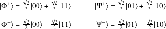
The entangled state we just used is known as a Bell state and there are four of them:
Question 8.2.2
Show that

Together, the four states |Φ+⟩, |Φ−⟩, |Ψ+⟩, and |Ψ−⟩ are an orthonormal basis for C2 ⊗ C2. They are named after John Stewart Bell, a physicist from Northern Ireland.
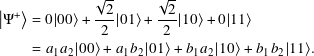
Let |Ψ⟩ be a 2-qubit quantum state in C2 ⊗ C2. |Ψ⟩ is entangled if and only if it cannot be written as the tensor products of two 1-qubit kets:
Suppose |Ψ+⟩ is not entangled. Then there exist a1, b1, a2, and b2 in C as above with
This gives us four relationships
Question 8.2.3
Is ![]() an entangled state?
an entangled state?
There is something I want to highlight that may be confusing at first. If we start with two 1-qubit states like a1 |0⟩1 + b1 |1⟩1 and a2 |0⟩2 + b2 |1⟩2 then we use all such tensor products (a1 |0⟩1 + b1 |1⟩1) ⊗ (a2 |0⟩2 + b2 |1⟩2) for all possible complex number coefficients to generate the state vector space C2 ⊗ C2.
This means we construct all possible sums of such tensor product forms. All the forms together do not constitute all of C2 ⊗ C2 but together with their sums they do.
Question 8.2.4
There is an infinite number of entangled states and an infinite number of separable states in C2 ⊗ C2. Given that, in what sense are there more entangled states than separable ones?
8.2.2 The general case
Every time we add a qubit to a quantum system to create a new one, the state space doubles in dimension. This is because we multiply the dimension of the original system’s state space by 2 when we do the tensor product. A 3-qubit quantum system has a state space of dimension 8. An n-qubit system’s state space has 2n dimensions.
Let n in N be greater than 1 and let Q be an n-qubit quantum system. The state space associated with Q has 2n dimensions. We write it as (C2)⊗n, which means C2 tensored with itself n times.
It is generated by the elementary tensor products of the 1-qubit states for each of the n qubits:
It’s much easier to use ket notation like |11010111⟩ than
The sets of n-qubit kets for (C2)⊗ n that are composed of only 0s and 1s are called computational bases. For example,
However we write the quantum state, the sum of the squares of the absolute values of the probability amplitudes add up to 1.
If we want to write a ket like
8.2.3 The density matrix again
If |ψ⟩ is a multi-qubit quantum state, its density matrix is defined in the same way as the 1-qubit case:

The diagonal elements are real, tr (ρ) = 1, and ρ is Hermitian and positive semi-definite. This means that ρ has a unique positive semi-definite square root matrix ρ1/2.
8.3 Multi-qubit gates
A quantum gate operation that operates on one qubit has a 2 by 2 unitary square matrix in a given basis. For two qubits, the matrix is 4 by 4. For ten, it is 210 by 210, which is 1024 by 1024. I show by example how to work with common lower dimensional gates and allow you to extrapolate to larger ones.
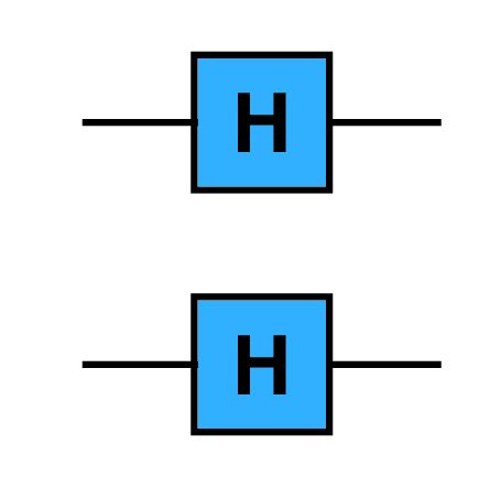
8.3.1 The quantum H⊗n gate
We start by looking at what it means to apply a Hadamard H to each qubit in a 2-qubit system. The H gate, or Hadamard gate, has the matrix


Though we could draw H⊗2 as having two inputs and two outputs, we instead show it by applying H to each qubit in a circuit.
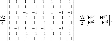
For a 3-qubit system, the corresponding H⊗3 matrix is

Question 8.3.1
Show that the normalization constant is 1/√2n where n is the number of qubits.
| 000 | 001 | 010 | 011 | 100 | 101 | 110 | 111 |
In contrast, the 3-qubit state H⊗3 |0⟩3 contains each of the corresponding ket basis forms at the same time.
This is a situation where the decimal expression for a basis ket is concise. We can rewrite the last equality as
The Hadamard gate matrices H⊗n can be defined recursively by
The general form for an n-qubit register state using decimal ket notation is
Question 8.3.2
Fully write out
8.3.2 The quantum SWAP gate
In subsection 7.6.1 we showed the X gate is a bit flip: given |ψ⟩ = a |0⟩ + b |1⟩, X |ψ⟩ = b |0⟩ + a |1⟩. Now that we are considering two qubits, is there a gate that switches the qubits? What does this even mean?
As we have seen before, given two qubits
The matrix


When I include the SWAP gate in a circuit it spans two wires. Remember the ×s!

8.3.3 The quantum CNOT / CX gate
The CNOT gate is one of the most important gates in quantum computing. It’s used to create entangled qubits. It’s not the only kind of gate that can do it, but it’s simple and very commonly used.
The ‘‘C’’ in CNOT is for ‘‘controlled.’’ Unlike the 1-qubit X gate, which unconditionally flips |0⟩ to |1⟩ and vice versa, CNOT has two qubit inputs and two outputs. Remember that quantum gates must be reversible. For this reason we must have the same number of inputs as outputs. We call the qubits q1 and q2 and their states |ψ⟩1 and |ψ⟩2, respectively.
This is the way CNOT works: it takes two inputs, |ψ⟩1 and |ψ⟩2.
- If |ψ⟩1 is |1⟩, then the state of q1 remains |ψ⟩1 but |ψ⟩2 becomes X |ψ⟩2.
- Otherwise the states of q1 and q2 are not changed.
Put another way, CNOT always operates like ID|ψ⟩1 for q1. When |ψ⟩1 = |1⟩, CNOT acts as X |ψ⟩2 for q2. Otherwise, it acts as ID |ψ⟩2. The CNOT is a conditional bit flip.
In the classical case, we create a controlled not from a xor with this circuit:

The matrix for CNOT is

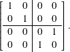
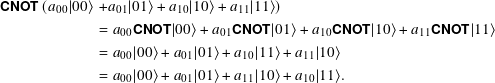
CNOT operates on the standard C2 ⊗ C2 basis as

| CNOT |00⟩ | = |00⟩ |
| CNOT |01⟩ | = |01⟩ |
| CNOT |10⟩ | = |11⟩ |
| CNOT |11⟩ | = |10⟩ . |
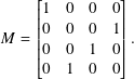
Applying the change-of-basis Hadamard H gates before and after CNOT illustrates an interesting property of CNOT. The matrix form of ![]() ○ CNOT ○
○ CNOT ○ ![]() is
is

If we wanted the control qubit to be the second one in this way, we would draw it with the • on the bottom. This is sometimes called a reverse CNOT.

CNOT is used to create the entangled Bell state vectors. We save the construction until subsection 9.3.2 when we have more of the circuit machinery in hand.
8.3.4 The quantum CY and CZ gates
The CNOT gate is the same as the CX gate. We can also create controlled 2-qubit gates for other 1-qubit gates. In block matrix form,

Question 8.3.3
What are the matrices for the CS and CH gates?

with the last two reversed to show that they can operate between arbitrary wires.
In general, if

Question 8.3.4
What is the matrix for the controlled-![]() , where
, where ![]() is defined in subsection 7.6.12 ?
is defined in subsection 7.6.12 ?
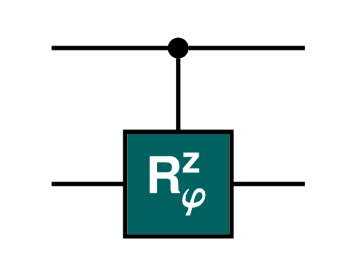
8.3.5 The quantum CRϕz gate
Another useful set of controlled gates are the ones where the action is ![]() . The first qubit controls whether the phase change, or rotation around the Bloch sphere z axis, should happen.
. The first qubit controls whether the phase change, or rotation around the Bloch sphere z axis, should happen.
The general matrix for ![]() is
is

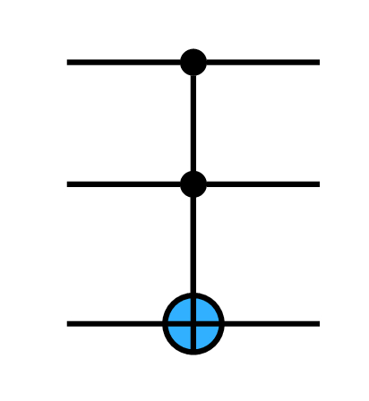
8.3.6 The quantum Toffoli CCNOT gate
The quantum Toffoli CCNOT gate is a double control gate operating on three qubits. If the states of the first two qubits are |1⟩ then it applies X to the third. Otherwise it is ID on the third. In all cases it is ID for the first two qubits.
Its matrix is an 8 by 8 permutation matrix which swaps the last two coefficients, like CNOT.

The Toffoli gate is also known as the CCX gate.
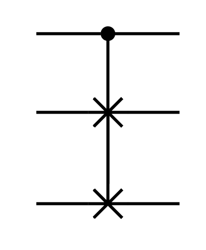
8.3.7 The quantum Fredkin CSWAP gate
The quantum Fredkin CSWAP gate is a control gate operating on three qubits. If the state of the first qubit is |1⟩ then the states of the second and third qubits are swapped, as in SWAP. If it is |0⟩, nothing is changed.
Its matrix is an 8 by 8 permutation matrix.

8.4 Summary
In this chapter we introduced the standard 2-qubit and 3-qubit gate operations to complement the classical forms from section 2.4. The CNOT gate allows us to entangle qubits. Entanglement, along with superposition and interference, is a key differentiator in quantum computing.
Now that we have a collection of gates, it’s time to put them into circuits and implement algorithms. We begin doing that in the next chapter.
References
- [1]
-
Paul R. Halmos. Finite-Dimensional Vector Spaces. 1st ed. Undergraduate Texts in Mathematics. Springer Publishing Company, Incorporated, 1993.
- [2]
-
W. Heisenberg. Across the frontiers. Ox Bow Press, 1990.
- [3]
-
S. Lang. Algebra. 3rd ed. Graduate Texts in Mathematics 211. Springer-Verlag, 2002.
- [4]
-
Saunders Mac Lane. Categories for the Working Mathematician. 2nd ed. Graduate Texts in Mathematics 5. Springer New York, 1998.