10
From Circuits to Algorithms
I am among those who think that science has great beauty.
Marie Curie
In the last chapter we became comfortable with putting together gates to create circuits for simple algorithms. We’re now ready to look at more advanced quantum algorithms and considerations on how and when to use them.
Our target in this chapter is Peter Shor’s 1995 algorithm for factoring large integers almost exponentially faster than classical methods. To get there we need more tools, such as phase estimation, the Quantum Fourier Transform, and function period finding. These are important techniques in their own rights, but are necessary in combination for quantum factoring.
We also return to the idea of complexity that we first saw for classical algorithms in section 2.8. This allows us to understand what ‘‘almost exponentially faster’’ means.
This chapter contains more mathematics and equations for quantum computing than we have encountered previously. I recommend that you take the time to understand the linear algebra and complex number computations throughout. While they may appear daunting at first, the techniques are used frequently in quantum computing algorithms.
Topics covered in this chapter
10.1.1 Roots of unity
10.1.2 The formula
10.1.3 The circuit
10.2 Factoring
10.2.1 The factoring problem
10.2.2 Big integers
10.2.3 Classical factoring: basic methods
10.2.4 Classical factoring: advanced methods
10.3 How hard can that be, again
10.4 Phase estimation
10.5 Order and period finding
10.5.1 Modular exponentiation
10.5.2 The circuit
10.5.3 The continued fraction part
10.6 Shor’s algorithm
10.7 Summary
10.1 Quantum Fourier Transform
The Quantum Fourier Transform (QFT) is widely used in quantum computing, notably in Shor’s factorization algorithm in section 10.6 . If that weren’t enough, the Hadamard H is the 1-qubit QFT and we’ve seen many examples of its use.
Most treatments of the QFT start by comparing it to the classical Discrete Fourier Transform and then the Fast Fourier Transform. If you don’t know either of these, don’t worry. I’m presenting the QFT in detail for its own sake in quantum computing. Should you know about or read up about the classical analogs, the similarities should be clear.
10.1.1 Roots of unity
We are all familiar with square roots. For example, √4 is equal to either 2 or −2. We can also write √2 = 21/2 and say that there are two ‘‘2nd-roots of 2.’’ Similarly, 5 is a cube root, or ‘‘3rd-root,’’ of 125. In general, we talk about an ‘‘Nth-root’’ for some natural number N. When we consider the complex numbers, we have a rich collection of such Nth-roots for 1.
Let N be in N. An Nth root of unity is a complex number ω such that ωN = 1. ‘‘ω’’ is the lowercase Greek letter ‘‘omega.’’ There are N Nth roots of unity and 1 is always one of those.
If every other Nth root of unity can be expressed as a natural number power of ω, then ω is a primitive Nth root of unity. If N is prime then every Nth root of unity is primitive except 1.
For N = 1, there is only one first root of unity, and that is 1 itself.
When N = 2, there are two second roots of unity: 1 and −1. −1 is primitive.
With N = 3, we can start to see a pattern. For this, remember Euler’s formula

and ω1 and ω2 are primitive.

For N = 4 we can do something similar, though the situation is much simpler.


Question 10.1.1
What are the primitive fourth roots of unity?
Notice something else here: for the first time, we see overlaps in the collection of roots of unity for different N. This happens when the greatest common divisor of the different N is greater than 1.
For N = 5 and above we continue in this way.
ω = e2π i/N is a primitive Nth root of unity.
When there is a fraction in the exponent of such expressions, it is common to pull the i into the numerator, as I have done here.
For some N as we have considered, let ω be an Nth root of unity. What is ω−1? This one is easy because
If ωk = e2π k i/N is a root of unity then
Question 10.1.2
Show that if ωk is a primitive Nth root of unity, so is ωk. Start by assuming that ωk is not primitive and see if that leads to a contradiction.
The polynomial xN − 1 can be factored as
For j and k in Z, the Kronecker delta function δj,k is defined by
Question 10.1.3
For a given N, let {ω0, ω1, …, ωN−2, ωN−1} be the Nth roots of unity. What is their product
To learn more
Roots of unity are an important concept and tool in several parts of mathematics, especially algebra [16] [8] and algebraic number theory [12] [19].
10.1.2 The formula
As we have seen, a general quantum state |ϕ⟩ on n qubits can be written
Definition
The quantum Fourier Transform of |ϕ⟩ is
For N = 2n and
Question 10.1.4
Show that QFTn is a linear transformation.
Question 10.1.5
Show that
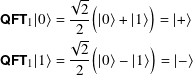
This is none other than H!
So QFT1 = H. Is QFTn = H⊗n?
No.
Matrix
From its definition, you can see that QFTn has matrix

- ω(N−1)(N−1) = ωN2 − 2N + 1 = ω because ωN2 = (ωN)N = 1N = 1.
- ωkN = ωN = 1 for k in Z.
- ω2(N−1) = ωN−2.
- ω−1 = ωN−1.
Applying rules such as these, we get
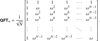
Question 10.1.6
Show that this is the matrix of QFTn and QFTn is unitary. For the latter, what is QFTn × QFTn†?

Recursive matrix
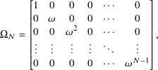
The higher Hadamard matrices H⊗n are defined recursively in terms of the lower ones by
- N = 2n,
- IN is the N by N identity matrix,
- ω is the primitive Nth root of unity e2π i/N,
- ΩN is the diagonal matrix
and
-
P2n+1 is a shuffle transform defined by setting its j, k entry via the formula
Remember that the first row and column index in the matrix is 1.
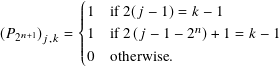
We do not derive this here but its effect is to move the vector entries with odd numbered indices to the front, followed by the even ones. For example,


Question 10.1.7
Compute P23.
10.1.3 The circuit
The QFT3 circuit can be constructed entirely from H, S, T, and SWAP gates. [20, Section 5.1]
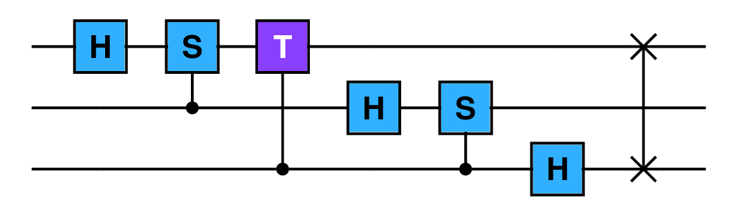
The last SWAP is necessary to reverse the order of the qubit quantum states. We can rewrite this with explicit ![]() gates.
gates.

An ![]() = S gate is a rotation given by the matrix
= S gate is a rotation given by the matrix

The pattern becomes clear when we extend this to 4 qubits and QFT4.

Question 10.1.8
Draw the circuit for 1 and 2 qubits. Using lots of ‘‘···’’, can you sketch the circuit for QFTn?
In this section we have discussed the Quantum Fourier Transform QFTn on n qubits. In some circuits we need the inverse Quantum Fourier Transform QFTn−1. We get this by running QFTn backwards. This is possible because all gates ultimately correspond to unitary operations, which are invertible and hence reversible.
Question 10.1.9
What is the defining matrix for QFTn−1?
For N = 2n and
To learn more
There is extensive literature about classical Fourier Transforms, particularly in engineering and signal processing texts. [4, Chapter 30] [10]
Quantum Fourier Transforms are used in many optimized quantum algorithms for arithmetic operations. [7] [25]
10.2 Factoring
It is hard to do a web search and find ‘‘practical’’ applications of factoring integers. Many of the results say things like ‘‘factoring integers is a tool in for factoring polynomials,’’ and ‘‘factoring integers is useful for solving some differential equations.’’ These examples are fine, but it seems like math to do more math.
One area where factoring comes into play is cryptography. There are cryptographic protocols that involve not being able to easily factor large numbers, in order to keep your information safe while it travels across the Internet or is stored in databases.
In this section, we examine some of the mathematics of factoring and focus in on one famous algorithm. This is Shor’s algorithm, named after its discoverer, mathematician Peter Shor. It can factor large integers almost exponentially faster than classical methods given a sufficiently large and powerful quantum computer.
If one does not understand what ‘‘sufficiently large and powerful’’ means, it is easy to make poor predictions of whether, or when, quantum computing can cause problems for encryption.
10.2.1 The factoring problem
Most people don’t worry about factoring integers once they graduate from high school or are no longer teenagers. In this book, we first encountered factoring when we discussed integers. In
As of this writing, the largest confirmed prime number has 24,862,048 digits. [21] Determining whether a number is prime or factoring that number are different but related problems. The part of mathematics that studies these topics, as well as many others, is called number theory.
While it can be hard to factor large integers, it is not simply the size that makes it difficult. The number
When we factor an N in Z greater than 1 we express it as a product
If n = 1 then N itself is prime. While the goal is to find all the pj factors, we really want to start by finding one pj and then continue by factoring the smaller integer N / pj. As we explore factoring, we focus on that first prime factor and then re-use our methods, basic or advanced, to do what’s left.
10.2.2 Big integers
On a 64 bit classical processor, the largest natural number you can represent is
What would you do if you wanted to factor 18,446,744,073,709,551,617, which is (264 − 1) + 2? The processor cannot hold the number directly in its hardware.
We fix this by creating ‘‘bignum’’ or ‘‘big integer’’ objects in software. These can be as large as computer memory permits. Essentially, we divide up the big integer across multiple hardware integers and then write software routines for negation, addition, subtraction, multiplication, division, and (related) quotients and remainders. Of these, the division operations are the trickiest to code correctly, though it is well known how to do it.
Scientific applications often support big integers. These include Maple, Mathematica, MATLAB®, and cryptographic software. Python, Erlang, Haskell, Julia, Ruby, and many variants of Lisp and Scheme are programming languages which provide built-in big integers. Other languages provide the functionality via library extensions.
The GNU Multiple Precision Arithmetic Library implements highly optimized low-level routines for arbitrary precision integers and other number types. It is distributed under the dual GNU LGPL v3 and GNU GPL v2 licenses. [9]
Let’s do a quick review of classical ways of factoring integers and then move on to Shor’s approach.
10.2.3 Classical factoring: basic methods
Classical factoring techniques can be broken down into basic attempts to break a number N down into prime factors that require arithmetic, and more advanced versions that require sophisticated mathematics. We go into detail on the former and survey the latter.
If N = 1 or N = −1, we are done. If N is negative, we note the unit is −1 and assume that N is positive.
There is one and only one even prime number and that is 2. If N is even, meaning that the last digit is one of 0, 2, 4, 6, or 8, then p1 = 2. Continue with N = N / 2. If this N is even, then p2 = 2, and reset N = N / 2. Keep going until N is not prime. If N ever becomes 1 in the factoring processes, we are done. At this point N is odd and we may have some initial pj factors equal to 2. To see if 3 is a factor we use a trick you may have learned while young.
Write N as a sequence of digits
Then N is divisible by 3 if and only if ![]() is.
is.
We can tell if 3 is a factor of N if 3 divides the much smaller integer that is the sum of the digits. To prove this, let N be as above. Then

Question 10.2.1
Clearly 100 ≡ 1 mod 3. Also, 101 ≡ 10 ≡ 32 + 1 ≡ 1 mod 3. Since a b mod 3 ≡ (a mod 3) (b mod 3), show that 102 ≡ 1 mod 3. How would you demonstrate that 10 j ≡ 1 mod 3?
There are no special tricks for 4 because we already factored out any 2s. 5 | N if the last digit is 0 or 5. Because 6 is 2 × 3, there is nothing to do.
For the prime 7 we can do trial division: divide N by 7 and if there is no remainder, 7 is a factor. There is nothing to do for 8, 9, or 10. For the prime 11 it is trial division again.
What I have described here is one mode of attack: start with a list of sorted primes and see if N is divisible by each in turn. You don’t need to look at all primes < N or even ≤ N/2, you need to look at those ≤ √N.
Question 10.2.2
If the prime p | N, p ≠ N, and p ≥ √N, why is there another prime q ≤ √N where q | N?
This is not a practical method of finding factors once N gets larger because division is computationally expensive and you have to do many of them. It’s not difficult to find what is called the integer square root of N, the largest integer s such that s2 ≤ N. This is ⌊√N⌋. If s2 = N then N is a square.
How would we go about creating a list of primes to use in trial division? A classical way (I really mean ‘‘classical’’ – it’s from ancient Greece) is the Sieve of Eratosthenes. Let’s see how this works to find all primes less than or equal to 30. We ‘‘sift’’ through the numbers and eliminate the composite values.
We begin by creating a list of all numbers in N less than or equal to 30. We underline all the numbers and selectively remove the underlines for the non-primes. We ‘‘mark’’ a number by removing its underline. When we are done, only the primes are underlined. Since 1 is not a prime, we mark it.
| 1 | 2 | 3 | 4 | 5 | 6 | 7 | 8 | 9 | 10 |
| 11 | 12 | 13 | 14 | 15 | 16 | 17 | 18 | 19 | 20 |
| 21 | 22 | 23 | 24 | 25 | 26 | 27 | 28 | 29 | 30 |
The first number that is not marked is 2. It must be prime. Now mark each of 2 + 2, 2 + 2 + 2, 2 + 2 + 2 + 2 and so on. The numbers we are marking are all multiples of 2 and so are not prime. We get:
| 1 | 2 | 3 | 4 | 5 | 6 | 7 | 8 | 9 | 10 |
| 11 | 12 | 13 | 14 | 15 | 16 | 17 | 18 | 19 | 20 |
| 21 | 22 | 23 | 24 | 25 | 26 | 27 | 28 | 29 | 30 |
After 2, the next number that is not marked is 3. It must be prime. We mark 3 + 3, 3 + 3 + 3, etc.
Question 10.2.3
Why would it be fine to start marking at 32 and then 32 + 3 instead of 3 + 3 and then 3 + 3 + 3?
| 1 | 2 | 3 | 4 | 5 | 6 | 7 | 8 | 9 | 10 |
| 11 | 12 | 13 | 14 | 15 | 16 | 17 | 18 | 19 | 20 |
| 21 | 22 | 23 | 24 | 25 | 26 | 27 | 28 | 29 | 30 |
After continuing in this manner, we end up with
| 1 | 2 | 3 | 4 | 5 | 6 | 7 | 8 | 9 | 10 |
| 11 | 12 | 13 | 14 | 15 | 16 | 17 | 18 | 19 | 20 |
| 21 | 22 | 23 | 24 | 25 | 26 | 27 | 28 | 29 | 30 |
The integers that remain are prime. This is not a terrible way to create a list of a few hundred or thousand primes, but you would not want to do this to find primes with millions of digits.
A simple Python implementation of the sieve is in Listing 10.1 . The output for the example above and a larger set of primes is
print(list_of_primes(30))

[2, 3, 5, 7, 11, 13, 17, 19, 23, 29]

print(list_of_primes(300))

[2, 3, 5, 7, 11, 13, 17, 19, 23, 29, 31, 37, 41, 43, 47, 53, 59, 61, 67,
71, 73, 79, 83, 89, 97, 101, 103, 107, 109, 113, 127, 131, 137, 139,
149, 151, 157, 163, 167, 173, 179, 181, 191, 193, 197, 199, 211, 223,
227, 229, 233, 239, 241, 251, 257, 263, 269, 271, 277, 281, 283, 293]
For a given number N, there are number theoretic algorithms such as the Miller-Rabin test if N is prime, or at least prime with high probability.
A further technique we can try is testing whether N is a power of another integer. Using an efficient algorithm called Newton’s method, we can determine whether N is an mth power. The most efficient method to do this test does so in O(log(N)) time. [1]
Which m do we need to try?
If 2m > N, then any other positive integer raised to the mth power is also too big. Therefore we need 2m ≤ N. By taking base 2 logarithms and noting that both sides are greater than one, we need to look at all m in Z such that
Another basic method is due to mathematician Pierre de Fermat. We can always represent N as the difference of two squares N = u2 − v2. The importance of this is that we then have
If we can find choices of u and v so that neither u + v nor u − v are 1, then we have a factorization.

Pierre de Fermat, 1601-1665. Image is in the public domain.
Another way of saying the above is
#!/usr/bin/env python3
def list_of_primes(n):
# Return a list of primes <= n using the Sieve of Eratosthenes
# Prepare the list of numbers containing [0,1,...,n]
numbers = list(range(n+1))
# Mark the first two numbers by setting them to 0
numbers[0] = numbers[1] = 0
# The first prime is 2
p = 2
# Cycle through the numbers, marking non-primes
while p < n:
if p:
index = p + p
while index <= n:
numbers[index] = 0
index += p
p += 1
# Return the primes left in the list
return [i for i in numbers if i != 0]
print(list_of_primes(30))
print(list_of_primes(300))
So is there a better alternative or approach?
Start by computing the integer square root s of N. If s2 = N we have found a factor. Otherwise, set u = s + 1 and consider u2 − N. If this is a square, then it is v2. If it is not, increment u by 1 and try again. Since N = (u + v)(u − v), we can stop when u + v ≥ n. (In fact, we can stop a little sooner, but this shows there is point after which we need not continue.)
Let’s try N = 143. s = 11 and since s2 ≠ 144, set u = s + 1 = 12. u2 − N = 144 − 143 = 1 and so set v = 1. v is a perfect square and so
This works well when a u + v and u − v are both close to √N. When they are not, we need to do many iterations and computations.
Question 10.2.4
Use Fermat’s method to factor 3493157. Use it again to factor 13205947.
10.2.4 Classical factoring: advanced methods
In Fermat’s method, we tried to find u and v such that
Given this, let g = gcd(u + v, N). Then g and N/g is a possible factorization of N. If either of these is 1 then we have failed and we have to find new candidates for u and v.
The key question is: how efficiently can we find u and v that are likely to work?
In Fermat’s method we work outwards from the integer square root of N, hoping to find a factor near it. Let’s briefly look at more advanced number theoretic approaches.
To learn more
The details are beyond the scope of this book but are well described elsewhere. [11] [15] [5]
Let B be in Z and ≥ 2. A positive integer is called B-smooth if all its prime factors are ≤ B. B is an upper bound on the size of the primes.
A factor base is a set P of prime numbers. Typically, given a bound B as above, P is the set of all primes ≤ B. If we simply say an integer n is smooth, we mean it is n-smooth, so it means all its prime factors are in P.
The following is known as Dixon’s method after its discoverer, mathematician John D. Dixon. For a given N to factor, choose B and hence P. Let n be the number of primes in P. We want to find n + 1 distinct positive integers fj such that j2 mod N is B-smooth. Said another way,
#import random

random.randint(5, 17)
returns a random integer greater than or equal to 5 and less than 17.
Now that we have our collection of fj, look at the product

- look for different fj, or
- increase B and keep trying.
Full treatments of the algorithm put bounds on the value of B. Can we find better congruences of squares, faster? The fj we use are smooth numbers. Can we sift through all the possibilities better so that we need not consider as many bad candidates?
To learn more
Beyond Dixon’s algorithm, there are more powerful and complicated number theoretic algorithms that generalize the sieving techniques to find smooth numbers much faster. The quadratic sieve and the general number field sieve are examples, with the latter being the most efficient factoring algorithm for very large integers. [2] [11, Chapter 3]
10.3 How hard can that be, again
In section 2.8 we first saw and used the O( ) notation for sorting and searching. Bubble sort runs in O(n2) time and merge sort is O(n log(n)). A brute force search is O(n) but adding sorting and random access allows a binary search to be O(log(n)). All algorithms are of polynomial time because we can bound them, in this case, by O(n2). More precisely, there is a hierarchy of time complexities. For the examples above,
| Algorithm | Complexity | Name |
| Bubble sort | O(n2) | quadratic time |
| Merge sort | O(n log(n)) | quasilinear time |
| Brute force search | O(n) | linear time |
| Binary search | O(log(n)) | logarithmic time |
Polynomial time is higher than all of them but we can say each runs in at least polynomial time.
We are concerned with this because there is a special distinction between polynomial time and exponential time. The latter describes exponential growth and can cause problems to become quickly intractable. All these descriptions apply to large n. Even though an exponential running time sounds bad, the algorithm may still be feasible when n is small.
Something running in exponential time has its execution time proportional to 2 f(n). Here f(n) is a polynomial in n such as n2 − n + 1. Double exponential time is even worse: the time is proportional to 2 2 f(n).
Subexponential is an improvement over exponential. It means for every b > 1 in R, the running time is less than bn. Set b = 2 to compare with exponential time. [13]
For example, an algorithm that runs in ![]() is subexponential.
is subexponential.
There are many subtleties concerning classical and quantum complexity, and a full discussion involves traditional and quantum Turing machines. As our need is only to understand where quantum computing can be better than classical computing, I don’t delve into a full and formal description of complexity theory here.
Fermat’s method of factoring integers is of exponential time. The general number field sieve is subexponential. There are no known polynomial time classical algorithms for factoring.
When you learned to add and multiply, you learned deterministic algorithms for each. Given the same input numbers, you executed a series of steps that always led to the same answer. No randomness was involved. If you encounter random numbers as you continue through this book, chances are you are looking at a non-deterministic algorithm.
A non-deterministic algorithm may involve probability and choices that could ultimately produce different answers. Even if the answers are the same, the choices made inside the algorithm may cause the algorithm to run quite quickly or excruciatingly slowly. More formally, a bad choice can cause an exponential time run while a good one can enable polynomial time execution.
The complexity class P refers to the collection of problems that can be solved in polynomial time using a deterministic algorithm.
The class NP is the collection of problems whose solutions can be checked in polynomial time. We do not know if P = NP but you could become wealthy via industry prizes if you could prove it or its contrary. Checking a solution by asking a question like ‘‘Is p × q equal to N?’’ is an example of a decision problem.
Consider integer factorization: we do not know if there is a classical way of factoring a composite integer in polynomial time but, once done, we can easily multiply together the factors to see if the solution is correct. Otherwise said, we do not know if classical factorization is in P but we know it is in NP.
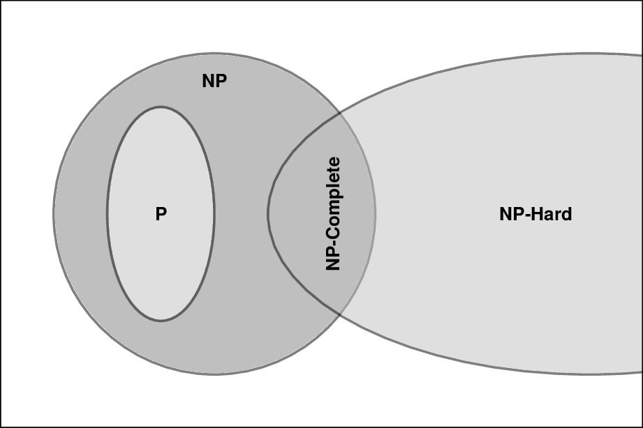
If P ≠ NP we can represent the set of problems as shown below. Not all NP problems are equally difficult. They are defined by their ability to check solutions in polynomial time.
Two new terms are shown: NP-Hard and NP-Complete. The first is easier to explain: the problems in NP-Hard are at least as hard as the most difficult ones in NP.
There is a valuable notion of reducing one problem to another. If A and B are two problems, we can ‘‘reduce A to B in polynomial time’’ if by a series of manipulations we can express A as an instance of B.
As an analogy, suppose one problem (A) is ‘‘travel to the Empire State building in New York City.’’ For problem B, we express it as ‘‘drive to any location in New York City.’’ B in general is hard because of the need to get to any location and the difficulty in driving to it. A can be reduced to B because we need to get to one location somehow.
A problem is in NP-Hard if any NP problem can be reduced to it. As you can see from the diagram, the class of NP-Hard problems intersects NP but is larger. The intersection is the NP-Complete class, the hardest problems in NP to which all others can be reduced. An NP-Hard problem that is not in NP cannot be solved or verified in polynomial time.
There are many, many (many, many, …) complexity classes that you may find interesting enough to learn more about beyond what we have discussed. BPP is the class of decision problems that can execute in polynomial time but with a caveat. BPP stands for ‘‘bounded-error probabilistic polynomial time.’’ Since probability is involved, an algorithm that solves this problem may not always return the correct answer. The ‘‘bounded’’ part of the name is made concrete by insisting the correct answer is gotten at least two-thirds of the time.
The class P is in BPP but it is not known if all problems in NP are in BPP.
The above classifications refer to problems solved on a classical computer. For quantum computers, we consider the BQP class, those solvable in bounded-error polynomial time on a quantum computer. BQP is short for ‘‘bounded-error quantum polynomial time.’’ Loosely speaking, BQP corresponds to quantum computers as BPP does for classical computers.
However, a stronger relationship exists. Any problem in BPP is also in BQP. This follows from our being able to perform classical operations on a quantum computer, though it might be extremely slow. We examined this in section 9.3 and subsection 9.3.1 when we saw that nand is universal for classical computing and we can create a nand on a quantum computer via a quantum Toffoli gate.
To learn more
A strong grounding in classical algorithms and complexity theory is necessary for you to become proficient in quantum algorithms. [4] [6] [26]
10.4 Phase estimation
Let U be an N by N square matrix with complex entries. From section 5.9 , the solutions λ of the equation
Each eigenvalue λj corresponds to an eigenvector vj so that
When U is unitary, we can say even more: each λj has absolute value 1 and so can be represented as
Now we are ready to pose the question whose solution we outline in this section:
Let U be a quantum transformation/gate on n qubits with corresponding N by N square matrix U, with N = 2n. If |ψ⟩ is an eigenvector of U (and of U, by abuse of notation), can we closely estimate ϕ where e2π ϕ i is the eigenvalue corresponding to |ψ⟩?
Some authors call the eigenvector |ψ⟩ an eigenket. I don’t in this book.
We are looking for a fractional approximation to ϕ. By increasing the number of qubits we use in the circuit, we can get a closer fit to ϕ.
Suppose U, |ψ⟩, and e2π ϕ i are as above. By applying U multiple times

If k = 2 j then ![]() .
.
We use this in the circuit for phase estimation in the following way.
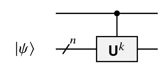
This is a controlled-Uk gate. The  indicates |ψ⟩ is represented on an n qubit register and Uk takes n quantum state inputs and outputs. This Uk is only run if the input on the wire above it is |1⟩.
Let U be a single qubit gate that operates like

Note how the value of the control qubit is modified.
Question 10.4.1
Show this is true via matrices and the standard basis kets.
This extends to larger matrices acting as a unit multiple of the identity and is exactly the case for how U operates on its eigenvector |ψ⟩.
Let m be the number of bits we need to get us as close as we need to the original phase. [20, Section 5.2] We use m qubits on the upper portion of the circuit, the ‘‘upper register.’’
When m = 2, our phase estimation circuit is

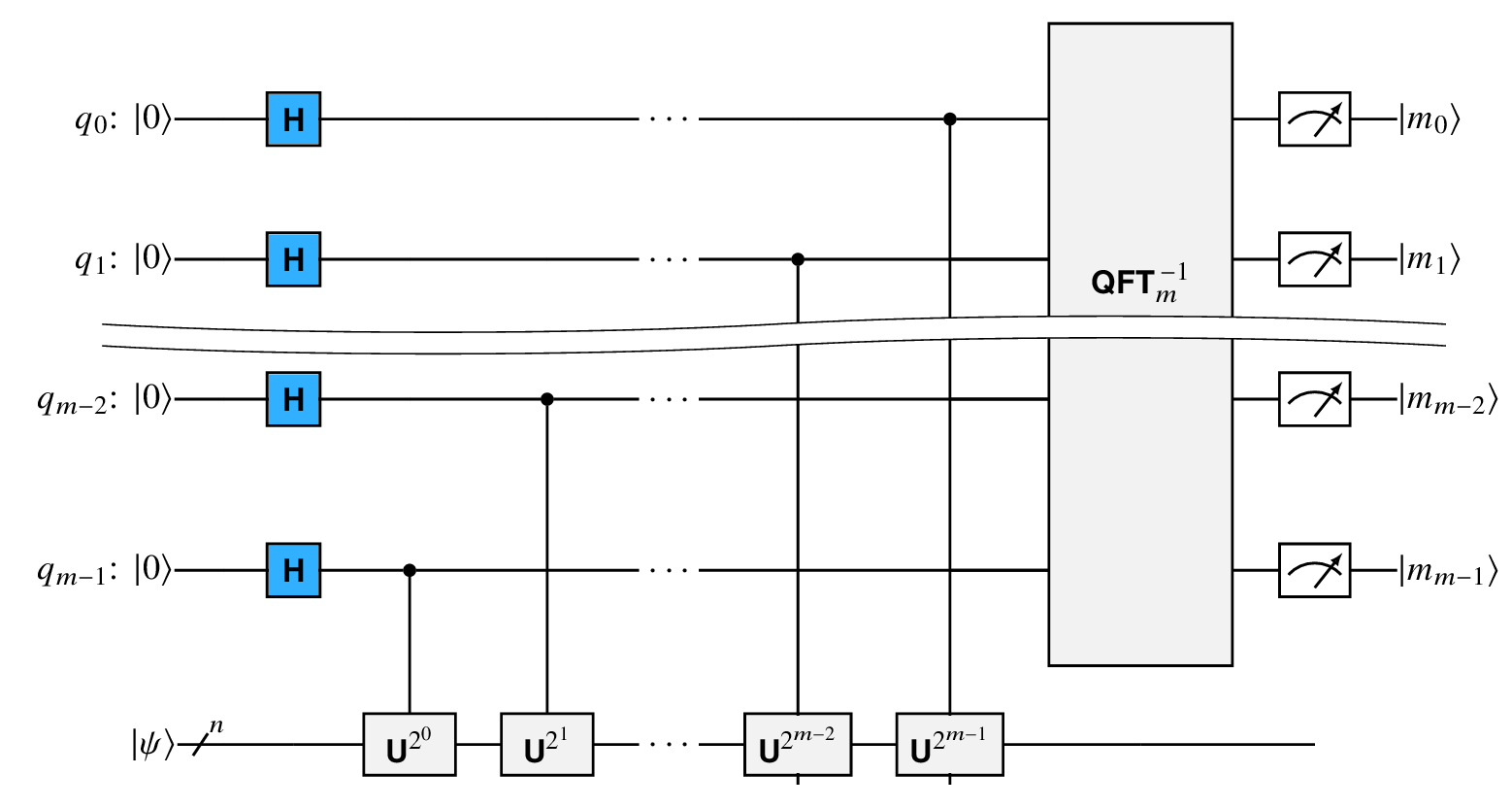
In general, we keep adding gates on the bottom up to U2m−1 as is shown in Figure 10.1. By the nature of application of the phase shifts described above, these modify the quantum states in the upper register. We then take the inverse Quantum Fourier Transform.
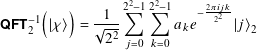
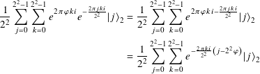
Continuing with our 2-qubit case, the state of the upper register before applying QFT2−1 is

I’ve highlighted two of the terms in the exponents to show the pattern.
In the 2-qubit case,


Obvious, right? Let me state why we have some of the elements in these messy expressions that we do:
- ϕ is the phase we want to estimate.
- The |j⟩2 are the standard basis kets.
- The sums involving the |j⟩2 are from superpositions.
- The exponential forms involving e are roots of unity or other complex numbers with absolute value 1.
- The QFTn−1 introduces the minus sign into the exponent while using QFTn would not have.
While the expressions look complicated, because they are, each part is there because of some gate action.
The general form of the last expression for m qubits instead of 2 is
Given c and d, we rewrite the upper register quantum state as

This means we must run the circuit multiple times to get the correct answer. If you run the circuit 28 or more times, the probability of never having gotten the correct answer is less than 10−6, as we saw in section 6.3 .
10.5 Order and period finding
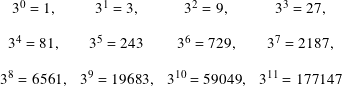
Consider the function ak on whole numbers k for a fixed a in N greater than 1. For example, if a = 3 then the first 12 values are
Question 10.5.1
What happens when we work modulo M = 23, 24, and 25?
For M = 13 in the first example, the period r = 3. For M = 16, r = 4. In the final example with M = 22, the period r = 5.
Given such an a as above, we can look at all a1, a2, a3, … modulo M and ask: what is the smallest r in N, if it exists, such that ar ≡ 1 mod M? If there is such an r, it is called the order of a mod M. Then ax+r ≡ ax mod M by multiplication by ax. Thus r is also the period of fa. For this reason, the ‘‘period finding problem’’ is equivalent to the ‘‘order finding problem.’’
In the rest of this section we develop a hybrid quantum-classical algorithm to find the order of such an a, with a few conditions.
This is an important algorithm because one of its applications is integer factorization. With such an r in hand, and assuming it is even,
Given a good a, a good even r, and Euclid’s algorithm, we might be able to find a factorization of M.
Now set
We use phase estimation with some post-processing using continued fractions to compute the order r of a modulo M. For 0 ≤ j ≤ r−1, we find approximations to the phases ϕj = j/r accurate to 2ℓbits + 1 bits with probability ≥ (1−ε)/r. The smaller our ε, the larger our ℓε is.
I’ve chosen to use ℓ to remind us that ℓbits and ℓε are lengths of quantum registers.
To learn more
In what follows, I generally follow the approach in Nielsen and Chuang, though there are many variations in the literature such as in Watrous, ideas of which are reflected here. [20, Section 5.3.1] [29]
10.5.1 Modular exponentiation
Since we are finding periods of functions or orders of numbers modulo M, we need to be able to compute ax mod M in a quantum way.
For a binary string y of length ℓbits, that is, y is in {0, 1}ℓbits, define
When I write an expression like |j mod M⟩ it is shorthand for |j mod M⟩ℓbits.
The |y⟩ are the computational basis vectors in a 2ℓbits-dimensional vector space over C. U is a 2ℓbits by 2ℓbits square matrix. The lower right 2ℓbits − M by 2ℓbits − M submatrix is the identity matrix. The upper left M by M submatrix is a permutation matrix because a is invertible modulo M. All other matrix entries are zero. Hence all of U is a permutation matrix consisting of 0s and 1s, and and so is unitary.
If we apply U multiple times, we get multiplication and hence exponentiation by repeated squaring:

As we saw at the end of section 9.4, for any non-negative integer z with binary representation zk−1 zk−2 ··· z1 z0 with z0 the least significant bit,

With these observations and calculations, we know how to do quantum modular exponentiation. Like many such quantum subroutines, we may need additional qubits for the computations outside the main circuit description. As in section 9.4, we can do modular exponentiation in O(ℓbits3) gates using algorithms similar to the simple classical versions.
We have one last thing to observe about U before we move on to the circuit for order finding and its analysis. With r the order of a modulo M, the kets

Question 10.5.2
Remembering that r is the order of a modulo M, show that
To learn more
Quantum Fourier Transforms are used in many optimized quantum algorithms for modular arithmetic operations. [24]
10.5.2 The circuit
To set up our circuit, we need two quantum registers. Since we use phase estimation, the first register needs enough qubits to get us the accuracy we need. This is ℓε. The number of qubits in the second register is ℓbits.
The circuit for the quantum portion of the order finding algorithm is in Figure 10.2 . The part of the circuit that I have labeled UPE is the core of the setup for the phase estimation. Referring back to the general phase estimation circuit in Figure 10.1, UPE needs to prepare an eigenvector in the second register and handle the controlled U2j gates.
Unfortunately, there is nothing that allows us to create


The value |1⟩ℓbits is not |111···111⟩ℓbits but is the ket |000···001⟩ℓbits, assuming the right-most bit is the least significant.
So while we cannot prepare an individual eigenvector |wj⟩, it is simple to prepare |1⟩ℓbits as the circuit below.

This is the first part of UPE for the lower quantum register. The rest of UPE is the sequence of controlled-U2j gates from Figure 10.1 .
Unlike the phase estimation algorithm, we are using a superposition of eigenvectors instead of a single one as the input to the lower quantum register. We’re not done, because what comes out of our circuit after applying the inverse QFT requires more work to get to r. In the next section, we use continued fractions to get us closer to the factorization.
10.5.3 The continued fraction part
We chose ℓε so that for 0 ≤ j ≤ r−1 we can find approximations ϕj to the phases j/r of U’s eigenvalues accurate to 2ℓbits + 1 bits with probability ≥ (1−ε)/r. j satisfies 0 ≤ j < r where each j is as probable as another. This is another way of saying that the j we get are uniformly distributed.
The output of the phase estimation algorithm after measurement is
If gcd(cj, 2ε) ≠ 1 then we try again because the fraction is not in reduced form. If cj and 2ε are coprime, we test if
We might just get a bad result with cj/2ε being, essentially, garbage. In this case, we can try again or decrease ε, thereby increasing ℓε.
We now employ this result about approximations and continued fractions:
Let a/b be a rational number in reduced form. Every reduced rational number c/d that satisfies
This statement is quite powerful: given two rational numbers, if the second is sufficiently close to the first, then the second is a convergent of the first. Reworking this for our situation gives the following result.
By our choice of ℓbits and ℓε, every reduced rational number ϕj = cj/2ε that satisfies
If cj/2ε is a good approximation to j/r then it is accurate to 2ℓbits + 1 bits with probability ≥ (1−ε)/r. What does it mean for some x to be accurate to some y for some number of bits b? Simply that
The complexity of the overall algorithm is dominated by the quantum modular exponentiation and so is O(ℓbits3).
10.6 Shor’s algorithm
We now have the tools we need to sketch Shor’s algorithm for factoring integers in polynomial time on a sufficiently large quantum computer.
The complete algorithm has both classical and quantum components. Work is done on both kinds of machines to get to the answer. It is the quantum portion that drops us down to polynomial complexity in the number of gates by use of phase estimation, order finding, modular exponentiation, and the Quantum Fourier Transform.
Let odd M in Z be greater than 3 for which you have already tried the basic tricks from subsection 10.2.3 to check it is not a multiple of 3, 5, 7, and so on. So that you don’t waste your time, you should also try trial division using a small list of primes, though this is not necessary. It is necessary, however, to make sure that M is not a power of a prime number, and you can use Newton’s method to test this.
So M is an odd positive number in Z that is not a power of a prime. It has a reasonable chance of being composite.
The following is the general approach to Shor’s algorithm given M as above:
- Choose a random number a such that 1 < a < M. Keep track of these values since we might need to repeat this step again.
- Check if gcd(a, M) = 1. If not, we have found a factor of M and we are done. This is pretty unlikely but now we know that a and M are coprime: they have no integer factors in common.
- Now find the non-zero order r of a mod M. This means that ar ≡ 1 mod M. If r is odd, go back to step 1 and try again with a different a.
- If r is even, we have
ar ≡ 1 mod M ⇒ ar − 1 ≡ 0 mod M ⇒ (ar/2 − 1) (ar/2 + 1) ≡ 0 mod M - Now look at gcd(ar/2 − 1, M) and, if necessary, gcd(ar/2 + 1, M). If either of these does not equal 1, we have found a factor of M and we have succeeded.
- If both of these greatest common divisors are 1, we repeat all the above from step 1 with another random a. We continue to do this until we find a factor.
To learn more
Other more advanced treatments go into the full complexity analysis and number theory behind this algorithm, starting with Shor’s original paper. [27] [17, Chapter 12] [18, Chapter 3] [23, Chapter 5]
In 2001, IBM Research scientists demonstrated factoring the number 15 via Shor’s algorithm on a 7-qubit NMR quantum computer. [28]
10.7 Summary
In this chapter we did some hard math to ultimately understand how to factor integers much faster than we can classically. Along the way we went deeply into several non-trivial quantum algorithms that are used in other quantum applications. These algorithms include the Quantum Fourier Transform, phase estimation, and order finding. These form a good basis for you to understand other quantum algorithms and their circuits.
We next turn our attention to the connections between the slightly abstract concepts we have seen so far and the physical quantum computers that we can build today.
To learn more
There are many other quantum algorithms though we have covered several of the most common ones. Techniques such as order finding are part of advanced algorithms in addition to Shor’s factorization. [3] [17] [22].
References
- [1]
-
Daniel J. Bernstein. ‘‘Detecting Perfect Powers in Essentially Linear Time’’. In: Mathematics of Computation 67.223 (July 1998), pp. 1253–1283.
- [2]
-
David M. Bressoud. Factorization and primality testing. Undergraduate Texts in Mathematics. Springer-Verlag New York, 1989.
- [3]
-
Patrick J. Coles et al. Quantum Algorithm Implementations for Beginners. 2018. url: https://arxiv.org/abs/1804.03719.
- [4]
-
Thomas H. Cormen et al. Introduction to Algorithms. 3rd ed. The MIT Press, 2009.
- [5]
-
R. Crandall and C. Pomerance. Prime Numbers: a Computational Approach. 2nd ed. Springer, 2005.
- [6]
-
Sanjoy Dasgupta, Christos H. Papadimitriou, and Umesh Vazirani. Algorithms. McGraw-Hill, Inc., 2008.
- [7]
-
Thomas G. Draper. Addition on a Quantum Computer. 2000. url: https://arxiv.org/abs/quant-ph/0008033.
- [8]
-
D. S. Dummit and R. M. Foote. Abstract Algebra. 3rd ed. Wiley, 2004.
- [9]
-
Free Software Foundation. The GNU Multiple Precision Arithmetic Library. url: https://gmplib.org/.
- [10]
-
R.W. Hamming. Numerical Methods for Scientists and Engineers. Dover Books on Engineering. Dover, 1986.
- [11]
-
Jeffrey Hoffstein, Jill Pipher, and Joseph H. Silverman. An Introduction to Mathematical Cryptography. 2nd ed. Undergraduate Texts in Mathematics 152. Springer Publishing Company, Incorporated, 2014.
- [12]
-
Kenneth Ireland and Michael Rosen. A Classical Introduction to Modern Number Theory. 2nd ed. Graduate Texts in Mathematics 84. Springer-Verlag New York, 1990.
- [13]
-
Burt Kaliski. ‘‘Subexponential Time’’. In: ed. by Henk C. A. van Tilborg and Sushil Jajodia. Springer US, 2011, pp. 1267–1267. url: https://doi.org/10.1007/978-1-4419-5906-5_436.
- [14]
-
A. Ya. Khinchin. Continued Fractions. Revised. Dover Books on Mathematics. Dover Publications, 1997.
- [15]
-
Neal Koblitz. A Course in Number Theory and Cryptography. 2nd ed. Graduate Texts in Mathematics 114. Springer-Verlag, 1994.
- [16]
-
S. Lang. Algebra. 3rd ed. Graduate Texts in Mathematics 211. Springer-Verlag, 2002.
- [17]
-
Richard J. Lipton and Kenneth W. Regan. Quantum Algorithms via Linear Algebra: A Primer. The MIT Press, 2014.
- [18]
-
N. David Mermin. Quantum Computer Science: An Introduction. Cambridge University Press, 2007.
- [19]
-
S.J. Miller et al. An Invitation to Modern Number Theory. Princeton University Press, 2006.
- [20]
-
Michael A. Nielsen and Isaac L. Chuang. Quantum Computation and Quantum Information. 10th ed. Cambridge University Press, 2011.
- [21]
-
Joe Palca. The World Has A New Largest-Known Prime Number. url: https://www.npr.org/2018/12/21/679207604/the-world-has-a-new-largest-known-prime-number.
- [22]
-
A.O. Pittenger. An Introduction to Quantum Computing Algorithms. Progress in Computer Science and Applied Logic. Birkhäuser Boston, 2012.
- [23]
-
Eleanor Rieffel and Wolfgang Polak. Quantum Computing: A Gentle Introduction. 1st ed. The MIT Press, 2011.
- [24]
-
Rich Rines and Isaac Chuang. High Performance Quantum Modular Multipliers. 2018. url: https://arxiv.org/abs/1801.01081.
- [25]
-
Lidia Ruiz-Perez and Juan Carlos Garcia-Escartin. Quantum arithmetic with the Quantum Fourier Transform. May 2017. url: https://arxiv.org/abs/1411.5949.
- [26]
-
Robert Sedgewick and Kevin Wayne. Algorithms. 4th ed. Addison-Wesley Professional, 2011.
- [27]
-
Peter W. Shor. ‘‘Polynomial-Time Algorithms for Prime Factorization and Discrete Logarithms on a Quantum Computer’’. In: SIAM J. Comput. 26.5 (Oct. 1997), pp. 1484–1509.
- [28]
-
Lieven M. K. Vandersypen et al. ‘‘Experimental realization of Shor’s quantum factoring algorithm using nuclear magnetic resonance’’. In: Nature 414.6866 (2001), pp. 883–887.
- [29]
-
John Watrous. CPSC 519/619: Introduction to Quantum Computing. url: https://cs.uwaterloo.ca/~watrous/LectureNotes/CPSC519.Winter2006/all.pdf.