3
Sub-classes of Functions
In the previous chapter, we defined the dioid of (min,plus) functions and studied its properties from an algebraic viewpoint. We also stressed several sub-classes such as functions that are non-decreasing and null at the origin. Indeed, the cumulative processes and curves we use in this book belong to this class.
In this chapter, we will investigate some properties of the (min,plus) operations from a calculus and analysis viewpoint. In particular, we will study more restricted sub-classes of functions. First, there are some shapes of functions that are very frequently encountered, such as leaky-buckets or rate-latency functions, and the (min,plus) operations can be computed very efficiently for these functions. This will be the purpose of section 3.1.
Next, in section 3.2, we will focus on the properties of the functions, such as the continuity and the monotony. Indeed, we saw in Chapter 1 that cumulative flows are modeled by non-decreasing, left-continuous functions, representing a cumulative amount of data. We will in particular focus on cases where the infimum of the (min,plus) convolution is in fact a minimum.
Finally, we will focus on concave and convex functions. These classes of functions are also widely used and, in Chapter 4, we will demonstrate that the (min,plus) operators can be efficiently implemented for these classes of functions.
A mathematical background about monotony and continuity can be found in the Appendix.
3.1. Usual functions
Several types of functions are commonly used in network calculus. In this section, we define these functions and use them to illustrate the computation of the (min,plus) operators – the convolution, the deconvolution and sub-additive closure – defined in Chapter 2. These examples will be used as illustrations of the notions that we will introduce in this chapter and the following ones.
DEFINITION 3.1 (Classes of usual functions).–
- 1) For all
 , the pure delay d is defined by
- 2) For all
 , the guaranteed rate R is defined by
  .
. - 3) For all
 , the rate-latency is defined by
  .
. - 4) For all
 , the token-bucket is defined by
  .
. - 5) For all
 and
and  , the staircase function is defined by
 , where
  .
. - 6) For all
 , the test function is defined by
Note that when ![]() , the zero element of the dioid and that
, the zero element of the dioid and that ![]() , the unit element (see Definition 2.3). We also have the following relations:
, the unit element (see Definition 2.3). We also have the following relations: ![]()
![]() . The staircase function
. The staircase function ![]() is sometimes denoted as
is sometimes denoted as ![]() when J is null. Note that unlike the other parameters, J can take negative or positive values. A positive value shifts the curve to the left, whereas a negative value shifts the curve to the right, as illustrated in Figure 3.1.
when J is null. Note that unlike the other parameters, J can take negative or positive values. A positive value shifts the curve to the left, whereas a negative value shifts the curve to the right, as illustrated in Figure 3.1.

Figure 3.1. Usual functions. For a color version of this figure, see www.iste.co.uk/bouillard/calculus.zip
All of these functions are piecewise continuous and left-continuous. They are also null at 0 (except ![]() with d < 0). In addition,
with d < 0). In addition, ![]() and
and ![]() are continuous.
are continuous.
PROPOSITION 3.1 (Sub/super-additivity of usual functions).–
- 1) For all
 is super-additive and
  .
. - 2) For all
 is both sub- and super-additive and
  .
. - 3) For all
 is super-additive and
 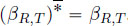 .
. - 4) For all
 is sub-additive and
- 5) For all
 and all
  is sub-additive and
 .
. - 6) For all
 and all
  is super-additive and
 .
.
Note that, except for the specific case of ![]() , the function
, the function ![]() is neither sub-additive nor super-additive.
is neither sub-additive nor super-additive.
PROOF.– From Definition 2.10, a sub-additive function satisfies for all ![]()
![]() and a super-additive function such that
and a super-additive function such that ![]()
![]() . We only need to show the sub/super-additivity as all those functions are null at 0. Lemma 2.6 and its equivalent with the super-additive closure in the (max,plus) setting allow us to conclude:
. We only need to show the sub/super-additivity as all those functions are null at 0. Lemma 2.6 and its equivalent with the super-additive closure in the (max,plus) setting allow us to conclude:
- 1) For all
 .
. - 2) Will be deduced from 3) and 4) using
 .
. - 3) For all
 , if
, if  , then
  . If
. If  , then
- 4) For all
 , if s = 0, then
  . If s > 0, then
  .
. - 5) First, as
 is sub-additive, so is
  . Second, if f is a sub-additive and non-decreasing function, so is
  for
for  . Indeed,
  . Therefore,
  is sub-additive for
  .
. - 6)
 is super-additive:
  . Moreover, if f is a sub-additive and non-decreasing function, so is
 . Thus, finally,
  and
and  for
for  are super-additive.
□
PROPOSITION 3.2 (Convolution and deconvolution by pure delays).– Let ![]() be a non-decreasing function, and
be a non-decreasing function, and ![]() . Then,
. Then,
In other words, convolution and deconvolution by pure delay functions are time-shifts.
PROOF.– For all ![]() If
If ![]() , then for all
, then for all ![]()
On the other hand, if ![]()
![]() , hence
, hence ![]() .
.
Let us now compute the deconvolution of f by ![]() . For all
. For all ![]()
![]() . Therefore,
. Therefore, ![]()
![]() . On the other hand,
. On the other hand, ![]()
![]() . Finally, we have
. Finally, we have ![]() .
.
□
PROPOSITION 3.3 (Sub-additive functions and pure delays).– Let ![]() be a
sub-additive function, and
be a
sub-additive function, and ![]() . Then,
. Then,
PROOF.– From Corollary 2.1, we have ![]() . We now have
to prove that
. We now have
to prove that ![]() is sub-additive. As f is non-negative,
is sub-additive. As f is non-negative, ![]() . Let
. Let![]()
![]() .
.
□
3.1.1. Convolution and deconvolution of the usual classes of functions
PROPOSITION 3.4 (Catalog of convolutions).–
- 1) For all

- 2) For all
 .
. - 3) For all
 .
. - 4) For all
 .
. - 5) For all
 .
.
No expression involving a staircase function is given since no simple analytic expression exists. To handle such curves, we may prefer to use algorithms which will be presented in Chapter 4. The convolution of a staircase function by a guaranteed rate is illustrated in Figure 3.2.

Figure 3.2. Convolution and deconvolution of a staircase function. For a color version of this figure, see www.iste.co.uk/bouillard/calculus.zip
PROOF.– 1) and 2) are direct applications of Proposition 3.2.
3) For all ![]() .
.
4) ![]() .
.
5) From Proposition 3.1, ![]() and
and ![]() . Then, from Proposition 2.6,
. Then, from Proposition 2.6, ![]() , and it is enough to prove that
, and it is enough to prove that ![]() is sub-additive (trivially
is sub-additive (trivially ![]() . Without loss of generality, we can assume that
. Without loss of generality, we can assume that ![]() and
and ![]() (the other cases are symmetric or such that
(the other cases are symmetric or such that ![]() is either smaller or greater than
is either smaller or greater than ![]() ). There exists a unique t0 > 0 such that
). There exists a unique t0 > 0 such that ![]() . For all
. For all ![]() and for all
and for all ![]() ,
, ![]() . Let
. Let ![]() . If
. If ![]() , then
, then ![]() . The same holds for
. The same holds for ![]() with
with ![]() replaced by
replaced by ![]() . Suppose that
. Suppose that ![]() . Then
. Then ![]() .
.
□
Before introducing the catalog of deconvolution, let us define the linear function ![]() . Note that
. Note that ![]() , leading, from Proposition 2.1, to
, leading, from Proposition 2.1, to ![]() .
.
PROPOSITION 3.5 (Catalog of deconvolutions).–
- 1) For all
 .
. - 2) For all
 .
. - 3) For all
 .
. - 4) For all
 .
. - 5) For all
 .
. - 6) For all
 .
.
As in the catalog of the convolution, no expression involving a staircase function is given. An illustration is shown in Figure 3.2.
PROOF.– 1), 2) and 3) are direct applications of Proposition 3.2.
4) and 5) are a direct consequence of 6), by taking T = 0 and b = 0.
6) From the definition of the deconvolution, for all ![]()
![]() . As
. As ![]() is non-decreasing and
is non-decreasing and ![]() for all u < T, we can write
for all u < T, we can write ![]()
![]() .
.
The supremum is obtained for u = T when ![]() , hence
, hence ![]()
![]() . On the other hand, if
. On the other hand, if ![]()
![]() and
and ![]() .
.
□
3.1.2. Horizontal and vertical deviations for the usual classes of functions
Let us first recall from Definition 1.5 the horizontal and vertical deviations:

We can now note that ![]() .
.
In practice, pure delay functions play a very important role in network calculus. The following results are often used to have a fast implementation of horizontal deviation when the second argument is a pure delay function. We prove it formally although it is quite intuitive as shown in Figure 3.3.

Figure 3.3. Horizontal deviation and pure delay functions. For a color version of this figure, see www.iste.co.uk/bouillard/calculus.zip
PROPOSITION 3.6 (Horizontal deviation and pure delay functions).– For all ![]() , and
, and ![]() ,
,
PROOF.– For all ![]() and all u > d,
and all u > d, ![]() , so
, so ![]() , and
, and ![]() .
.
We will show a slightly stronger result than the second statement: the result holds if for all t > 0, f (t) > 0. Indeed, in that case, for all ![]() , so for all
, so for all ![]() . This is true for all
. This is true for all ![]() , so
, so ![]() , hence
, hence ![]() .
.
□
PROPOSITION 3.7 (Catalog of deviations).–
- 1) For all
 .
. - 2) For all
 .
. - 3) For all
 .
. - 4) For all
 .
.
PROOF.– 1) is the direct application of Proposition 3.6.
3) and 4) are direct applications of Proposition 3.5, using the relation hDev(f, g) = f ![]() g(0).
g(0).
![]() , so
, so ![]() = 0. For all t > 0,
= 0. For all t > 0,
So ![]() , and
, and ![]() , and +∞ otherwise.
, and +∞ otherwise.
□

Figure 3.4. Horizontal and vertical deviations for token-bucket and rate-latency functions. For a color version of this figure, see www.iste.co.uk/bouillard/calculus.zip
3.2. Non-negative and non-decreasing functions
Note that the set of non-negative and non-decreasing functions is ![]() . We have the following properties that are either proved in Chapter 2 or straightforward:
. We have the following properties that are either proved in Chapter 2 or straightforward:
- – if
 , then
  ;
; - – if
 and
and  , then
  .
.
However, we saw in Chapter 1 that some network calculus operations use subtraction, which does not preserve the monotonicity. In order to avoid this problem, and because it is consistent with the network calculus theory, we introduce some closure operators to remain in the set of non-negative and/or non-decreasing functions.
DEFINITION 3.2 (Non-negative and non-decreasing closures).– Let ![]() be a function. Its non-negative, non-decreasing and non-negative non-decreasing closures are, respectively, defined by
be a function. Its non-negative, non-decreasing and non-negative non-decreasing closures are, respectively, defined by
The semantics of ![]() clearly appears once the definition of the (max,plus) convolution is expanded:
clearly appears once the definition of the (max,plus) convolution is expanded: ![]() .
.
For example, the rate-latency function βR,T is the non-negative closure of linear function ![]() . An example of non-decreasing closure is shown in Figure 3.5.
. An example of non-decreasing closure is shown in Figure 3.5.

Figure 3.5. A function f and its non-decreasing closure  . For a color version of this figure, see www.iste.co.uk/bouillard/calculus.zip
It should be obvious that ![]() is the least non-negative function that is greater than or equal to
is the least non-negative function that is greater than or equal to ![]() . Let us prove a similar property for
. Let us prove a similar property for ![]() ; then it can also be deduced that
; then it can also be deduced that ![]() is the least function greater than or equal to
is the least function greater than or equal to ![]() that is both non-negative and non-decreasing.
that is both non-negative and non-decreasing.
LEMMA 3.1.– Let ![]() be a function. Then,
be a function. Then, ![]() is the least non-decreasing function greater than or equal to
is the least non-decreasing function greater than or equal to ![]() , i.e.
, i.e.
PROOF.– If s < t, then ![]() . Therefore,
. Therefore, ![]() is non-decreasing.
is non-decreasing.
Moreover, for all ![]() .
.
Finally, if there existed ![]() and t ∈
and t ∈ ![]() such that
such that ![]() , then, by definition of
, then, by definition of ![]() (t), there would exist s < t such that g(t) <
(t), there would exist s < t such that g(t) < ![]() . However, as
. However, as ![]() , g cannot be non-decreasing, hence the implication.
, g cannot be non-decreasing, hence the implication.
□

Figure 3.6. Pseudo-inverse of a function
3.2.1. Pseudo-inverse of a function
For a bijective function ![]() (especially when
(especially when ![]() is strictly increasing), inverse functions can be defined: for each value
is strictly increasing), inverse functions can be defined: for each value ![]() , there exists a unique t ∈
, there exists a unique t ∈ ![]() such that
such that ![]() , and we can set
, and we can set ![]() . However, in the network calculus context, we deal with functions that are only non-decreasing, so we have to deal with the notion of pseudo-inverse instead.
. However, in the network calculus context, we deal with functions that are only non-decreasing, so we have to deal with the notion of pseudo-inverse instead.
DEFINITION 3.3 (Pseudo-inverse).– Let ![]() be a non-negative and non-decreasing function. Then, pseudo-inverse
be a non-negative and non-decreasing function. Then, pseudo-inverse ![]() is defined by
is defined by ![]() ,
,
The definition of pseudo-inverse is illustrated in Figure 3.6. An inverse cannot be defined as for all t ∈ [2,3], ![]() = 2. With our definition,
= 2. With our definition, ![]() , and
, and ![]() . Note that other definitions of pseudo-inverse exist, for example, by replacing the non-strict inequality by a strict inequality. When considering two pseudo-inverses, two different notations must be used, like
. Note that other definitions of pseudo-inverse exist, for example, by replacing the non-strict inequality by a strict inequality. When considering two pseudo-inverses, two different notations must be used, like ![]() in [BOY 16] or
in [BOY 16] or ![]() in [LIE 17].
in [LIE 17].
Our choice has been driven by the preservation of the left-continuity of the function, as it will be proved in Proposition 3.8. First, Lemma 3.2 gives an alternative equivalent definition of the pseudo-inverse.
LEMMA 3.2.– Let ![]() be a non-decreasing function. Then, for all
be a non-decreasing function. Then, for all ![]() ,
,
Before proving this lemma, let us introduce a notation that will be used in the next two proofs: ![]() , where
, where ![]() . For example,
. For example, ![]() .
.
PROOF.– We have to prove that ![]() . First note that
. First note that ![]() form a partition of
form a partition of ![]() . Indeed, for all t ∈
. Indeed, for all t ∈ ![]() , either
, either ![]() (and t ∈
(and t ∈ ![]() ), or
), or ![]() . Moreover, as
. Moreover, as ![]() is non-decreasing,
is non-decreasing, ![]() is an interval of the form
is an interval of the form ![]() (it can be either open or closed on the left): if t ∈
(it can be either open or closed on the left): if t ∈ ![]() , then for all
, then for all ![]() , and by consequence,
, and by consequence, ![]() is an interval of the form
is an interval of the form ![]() . Finally,
. Finally, ![]() .
.
□
In the proof, we also showed that if ![]() is non-decreasing, then
is non-decreasing, then ![]() and
and ![]() .
.
PROPOSITION 3.8 (Pseudo-inverse properties).– Let ![]() be a non-negative and non-decreasing function, then:
be a non-negative and non-decreasing function, then:
- 1)
 .
. - 2) Pseudo-inversion relations: for all t ∈
 and all
  ,
,
- 3)
 is left-continuous.
PROOF.– 1) First, let ![]() be such that
be such that ![]() . Then
. Then ![]() , so
, so ![]() , and
, and ![]() is non-decreasing.
is non-decreasing.
Second, ![]() , so 0 ∈
, so 0 ∈ ![]() , and
, and ![]() , which is equivalent to
, which is equivalent to ![]() .
.
2) The first set of implications can be expanded to:
and the second set is the contraposition of the first set.
3) Fix ![]() . We have
. We have ![]() from Lemma 3.2 and let us denote
from Lemma 3.2 and let us denote ![]() . We want to show that for any increasing sequence
. We want to show that for any increasing sequence ![]() converging to
converging to ![]() converges to t. As
converges to t. As ![]() is non-decreasing, we have that, for all
is non-decreasing, we have that, for all ![]() , so (tn) is converging to some value
, so (tn) is converging to some value ![]() . Moreover,
. Moreover, ![]() .
.
Suppose that ![]() . Then, there exists s such that
. Then, there exists s such that ![]() < s < t. For all
< s < t. For all ![]() ,
, ![]() . The third implication comes from (3). As
. The third implication comes from (3). As ![]() converges to x, this means that
converges to x, this means that ![]() , and then
, and then ![]() .
.
□
PROPOSITION 3.9 (Catalog of pseudo-inverses).–
- 1) For all
 if
if  and
and  otherwise.
 - 2) For all d ∈
 .
. - 3) For all
 .
. - 4) For all R, T ∈
 R > 0.
The fact that the pseudo-inverse is idempotent (i.e. ![]() in these examples is not a general property, but due to the left-continuity of the functions, and their belonging to
in these examples is not a general property, but due to the left-continuity of the functions, and their belonging to ![]() . For example, the function
. For example, the function ![]() defined by
defined by ![]() and
and ![]() have the same pseudo-inverse.
have the same pseudo-inverse.
3.2.2. Convolution and continuity
In this section, we continue our investigations regarding the (left-)continuity of the function, with regard to the (min,plus) convolution. Indeed, the convolution is defined as an infimum, and one important problem that arises in network calculus is knowing whether that infimum is a minimum or not. Roughly speaking, for the convolution of ![]() and g, this would imply the existence of s such that
and g, this would imply the existence of s such that ![]() , and simplify the reasoning.
, and simplify the reasoning.
PROPOSITION 3.10 (Convolution infimum can be a minimum).– Let ![]() be two non-decreasing functions:
be two non-decreasing functions:
- 1) if
 and g are left-continuous, then ∀t ∈
  , ∃s ∈ [0, t] such that
- 2) if g is continuous, then ∀t ∈
 , ∃s ∈ [0, t] such that
  .
.
The proof of the first statement is taken from [BOU 11a, Lemma 1] and the second from [LEB 01, Th 3.1.8].
PROOF.– Note that if the functions are non-decreasing, ![]() exists for all x ∈
exists for all x ∈ ![]() (possibly +∞).
(possibly +∞).
- 1) Fix t ∈
 and define
  . Let (un) be a sequence such that F(un) is decreasing and converges to
  . As for all n un ∈ [0, t], a compact set, there exists a subsequence of (un) that converges. Let us denote this limit by u. Moreover, it is possible to extract from this subsequence another subsequence that is either increasing or decreasing. Let us assume that (un) is this subsequence and, without loss of generality, that it is also increasing (by exchanging the role of
  and g and replacing (un) by (t - un) if needed).
As
 is left-continuous,
  and, as g is left-continuous and non-decreasing, limn→∞ g(t - un)
  g(t - u). Then, limn→∞ F(un)
  F(u). As a result, F reaches its minimum on [0, t].
 - 2) The previous proof is modified as follows: consider a sequence (un) converging to u defined previously. Without loss of generality, (un) is either increasing or decreasing. If (un) is increasing, then
 and if (un) is decreasing, then
  . As g is continuous, then limn→∞ g(t - un) = g(t - u). Therefore, in any case, limn→∞ F(un)
  F(u-), and there exist sequences where F(u-) is reached ((un) = (u - 1/n), for example), hence the result.
□
PROPOSITION 3.11 (Continuity of the convolution).–Let ![]() be two non-decreasing functions. If
be two non-decreasing functions. If ![]() and g are left-continuous, then, so is
and g are left-continuous, then, so is ![]() * g.
* g.
PROOF.– For all s ∈ ![]() , define
, define ![]() . The left-continuity of Fs directly follows from that of g, and for all
. The left-continuity of Fs directly follows from that of g, and for all ![]() . The latter equality is because
. The latter equality is because ![]() is non-decreasing. Note that from Lemma 3.10, this is a minimum, and we denote one value by ut such that
is non-decreasing. Note that from Lemma 3.10, this is a minimum, and we denote one value by ut such that ![]() (if ut is not unique, it can be chosen arbitrarily).
(if ut is not unique, it can be chosen arbitrarily).
Fix t ∈ ![]() and (tn) a non-decreasing sequence converging to t. To prove the left-continuity of
and (tn) a non-decreasing sequence converging to t. To prove the left-continuity of ![]() at t, we need to show that
at t, we need to show that ![]() converges to
converges to ![]() , with
, with ![]() .
.
As in the previous proof, we can extract from (un) a converging and increasing sequence (by exchanging the roles of ![]() and g if needed), and then assume without loss of generality that (un) is increasing, and denote its limit by u. We have
and g if needed), and then assume without loss of generality that (un) is increasing, and denote its limit by u. We have ![]() where g+ is either g(t - u) or g(t - u+), depending on how tn - un is converging.
where g+ is either g(t - u) or g(t - u+), depending on how tn - un is converging.
On the other hand, from Lemma 2.3, ![]() is non-decreasing, so
is non-decreasing, so ![]() , and finally
, and finally ![]() .
.
□
3.3. Concave and convex functions
Most of the functions we defined in section 3.1 are concave or convex. For example, rate-latency and pure delay functions are convex and token-bucket functions are concave. These functions can also be combined so that we have to consider concave and convex functions (e.g. the minimum of token-buckets functions is a piecewise affine and concave function, and the maximum of rate-latency functions is a piecewise affine and convex function). In the remaining part of this chapter, we will focus on these two classes of functions.
3.3.1. Concave functions
We deal in this section with the concave functions, and we mainly state that concave functions are almost a sub-class of sub-additive functions defined in Chapter 2. Let us first recall the definition of a concave function:
DEFINITION 3.4 (Concave function).– A function ![]() is concave if and only if
is concave if and only if
Graphically, the arc drawn between two points of a concave function is below the function, as depicted in Figure 3.7. The interested reader may refer to [ROC 97] for a more complete reference to concave functions. Concave functions of ![]() are also continuous on
are also continuous on ![]() {0}.
{0}.

Figure 3.7. Concave function, with  and
and 
The next proposition states some useful properties of concave functions regarding the (min,plus) operators.
PROPOSITION 3.12 (Properties of concave functions).– Let ![]() , g be two concave functions. Then:
, g be two concave functions. Then:
- 1)
 + g is concave;
 - 2)
 ∧ g is concave;
 - 3) if
 is sub-additive;
 - 4)
 . In particular, if
  ;
; - 5) if
 , then
  .
.
We can deduce from these properties that the set of concave functions is a sub-dioid of ![]() (the zero and unit elements are concave).
(the zero and unit elements are concave).
These properties have a huge practical impact on computational aspects of network calculus. First, the computation of the convolution can be reduced to the computation of the minimum, which is usually a simpler operation to perform.
Note that sub-additive functions that are not concave do exist. For example, we can check that the function ![]() is sub-additive as
is sub-additive as ![]() , but is not continuous on (0, +∞), hence it is not concave.
, but is not continuous on (0, +∞), hence it is not concave.
Based on these properties, the class of concave piecewise linear functions will be presented in section 4.2.
- PROOF.– 1)
 ,
,

so
 + g is concave.
 - 2)
 ,
,

Similarly,
 . Therefore,
and
 ∧ g is concave.
 - 3) If
 , then for all t ∈
  and all
  . Now, for all s > 0, set
  and
and  , we can write

which proves that
 is sub-additive.
 - 4) First assume that
 (0) = g(0) = 0. We know that ∀t ∈
  and
and  ,
,  and qg(t)
  g(qt). Then,
  , and we can write, using p = s/t and q = (t – s)/t,

with equality when
 or
or  . Therefore,
 .
.In the general case, we have

and the result with
 and
and  can be applied.
 - 5) By Corollary 2.1,
 . But, f is concave and
  , so
, so 
 is also concave, hence sub-additive, and
  . Thus, by Lemma 2.6,
  .
.
□
3.3.2. Convex functions
The class of convex functions has different properties regarding the (min,plus) dioid. Indeed, convex functions are not stable by the minimum, hence they do not form a sub-dioid. However, an equivalent of the Fourier transform (the Legendre–Fenchel transform) can be defined, and the convolution corresponds to the addition in the space of the transforms, which will translate into efficient algorithms in Chapter 4. This also enables us to prove the stability of the convex functions by the convolution.
Let us first recall the definition of a convex function.
DEFINITION 3.5 (Convex function).– A function ![]() is convex if and only if
is convex if and only if
In other words, f is convex if and only if ![]() is concave and the next proposition is a direct consequence of Proposition 3.12. Moreover, we note that the functions that are both convex and concave are exactly the linear functions (satisfying
is concave and the next proposition is a direct consequence of Proposition 3.12. Moreover, we note that the functions that are both convex and concave are exactly the linear functions (satisfying ![]()
![]() .
.
The two first points of the next proposition are deduced using the duality of (min,plus) and (max,plus) dioids and Proposition 3.12.
PROPOSITION 3.13 (Properties of convex functions).– Let f and g be two convex functions of ![]() . Then:
. Then:
- 1)
 is convex;
 - 2)
 is convex;
 - 3)
 is convex.
PROOF.– For all ![]() and all
and all ![]() , with
, with ![]() ,
,

□
We are now ready to define the Legendre–Fenchel transform [ROC 97]. As already mentioned, it can be roughly seen as the equivalent of the Fourier transform in the classical algebra. However, as ![]() is not a field, the space where this transform in an involution is not the whole space
is not a field, the space where this transform in an involution is not the whole space ![]() . We will see that there is a close relation with convex functions. This transform has already been used in the network calculus literature to efficiently compute performance bounds [FID 06a] or in the context of a formal series of the idempotent semi-ring
. We will see that there is a close relation with convex functions. This transform has already been used in the network calculus literature to efficiently compute performance bounds [FID 06a] or in the context of a formal series of the idempotent semi-ring ![]() [BUR 03, COH 89].
[BUR 03, COH 89].
DEFINITION 3.6 (Legendre–Fenchel transform).– The Legendre–Fenchel transform of the space ![]() is the mapping
is the mapping ![]() defined by
defined by
The next proposition gives some examples of computations of Legendre–Fenchel transforms.
PROPOSITION 3.14 (Examples of Legendre–Fenchel transforms).–
- 1) For all
 .
. - 2) For all
 .
. - 3) For all
 .
.
PROOF.– 1) For all ![]() . If
. If ![]() , the supremum is reached for
, the supremum is reached for ![]() and
and ![]() ; if
; if ![]() is not bounded and
is not bounded and ![]() .
.
2) For all ![]() , since
, since ![]() .
.
3) For all ![]() . Similar to the first case, the supremum is unbounded when
. Similar to the first case, the supremum is unbounded when ![]() , and the supremum is obtained for
, and the supremum is obtained for ![]() when
when ![]() , so that
, so that ![]() .
.
□
Note that it is also possible to deduce (3) from (1) and (2) using the third property of the next result: the convolution corresponds to the addition in the transform space.
PROPOSITION 3.15.– ![]()
- 1)
 is convex and non-decreasing;
 - 2)
 ;
; - 3)
 ;
; - 4) if f is convex and non-decreasing, then
 .
.
PROOF.– 1) Let ![]() with
with ![]() . Then,
. Then, ![]()
![]() , so
, so ![]() is non-decreasing.
is non-decreasing.
Let ![]() and
and ![]() . Then,
. Then,

Thus, ![]() is convex.
is convex.
2) ![]()

3) ![]()

4) Let f be a convex and non-decreasing function of ![]() . First,
. First, ![]() . Indeed, for
. Indeed, for ![]() ,
,
Fix ![]() and we obtain that
and we obtain that ![]() .
.
Next, we need to show the equality. For this, let us introduce the concept of a supporting line. We say that f has a supporting line at ![]() of slope
of slope ![]() if
if ![]() , i.e. the affine function of slope α that meets f at x is below f. It should be obvious to an alert reader (if not, the reader can refer to [RoC 97] for the basic properties of convex functions) that a non-decreasing convex function has supporting lines at each point
, i.e. the affine function of slope α that meets f at x is below f. It should be obvious to an alert reader (if not, the reader can refer to [RoC 97] for the basic properties of convex functions) that a non-decreasing convex function has supporting lines at each point ![]() either f is differentiable at x and the slope is unique and equal to
either f is differentiable at x and the slope is unique and equal to ![]() , or f is not differentiable and the possible slopes form an interval. This interval is
, or f is not differentiable and the possible slopes form an interval. This interval is ![]() where
where ![]() and
and ![]() are respectively the left and right derivatives of f at x. Moreover, f can be characterized as the infimum of all its supporting lines. Now, if f has a supporting line at x of slope
are respectively the left and right derivatives of f at x. Moreover, f can be characterized as the infimum of all its supporting lines. Now, if f has a supporting line at x of slope ![]() , then
, then ![]() has a supporting line at
has a supporting line at ![]() of slope x. Indeed, on the one hand,
of slope x. Indeed, on the one hand, ![]()
![]() , as the minimum is reached for
, as the minimum is reached for ![]() . On the other hand, for any
. On the other hand, for any ![]() (taking
(taking ![]() ). Thus,
). Thus, ![]() .
.
Now, if ![]() has a supporting line at
has a supporting line at ![]() of slope x, then
of slope x, then ![]() has a supporting line at x of slope
has a supporting line at x of slope ![]() , and then
, and then ![]() and f has exactly the same set of supporting lines, so they are equal.
and f has exactly the same set of supporting lines, so they are equal.
□
We can see from points 2) and 3) of this proposition that ![]() is a (non-injective) homomorphism. Therefore, the following equivalence relation is a congruence, i.e. an equivalence relation compatible with operations
is a (non-injective) homomorphism. Therefore, the following equivalence relation is a congruence, i.e. an equivalence relation compatible with operations ![]() and
and ![]() of
of ![]()
Therefore, all functions that have the same Legendre–Fenchel transform belong to the same equivalence class modulo ![]()
Another consequence of the last point of this proposition is that ![]() is an involution over the sets of convex non-decreasing functions, and the convolution of two functions can be computed with the formula
is an involution over the sets of convex non-decreasing functions, and the convolution of two functions can be computed with the formula ![]() .
.
Note that, here, we only deal with non-decreasing functions. In fact, the result can hold in the more general framework of convex functions when the functions are defined on ![]() and not
and not ![]() (hence the result about the stability of convex functions regarding the convolution could be stated without the non-decreasing property).
(hence the result about the stability of convex functions regarding the convolution could be stated without the non-decreasing property).
3.4. Summary
Usual classes of functions

For a color version of this figure, see www.iste.co.uk/bouillard/calculus.zip
The main properties (Propositions 3.4 and 3.5) can be summarized by:

Non-negative and non-decreasing functions: ![]() is stable by
is stable by ![]()
Closure operators:

Pseudo-inverse: Lemma 3.2 and Propositions 3.9:
Concave function: concave functions are stable by ![]() .
.
f, g concave and ![]() and
and ![]() .
.
Convex functions: convex functions are stable by ![]() .
.
Legendre–Fenchel transform (Definition 3.6): ![]()
f convex and non-decreasing ![]() and
and ![]() .
.