From this chapter forward, we will start touching on the chunk options in knitr. First, in this chapter, we explain how to tune text output, including output from inline R code as well as text output from code chunks.
If the inline R code produces character results, they will be directly written into the output. When the result is numeric, scientific notation will be considered to denote the numbers that are too big or too small.
The threshold between scientific notation and fixed notation is the R option scipen (see ?options for details). By default (scipen = 0), if a positive number is bigger than 104 or smaller than 10−4 (this applies to the absolute values of negative numbers too), it will be denoted in scientific notation. Depending on the output format (![]() or HTML), knitr will use the appropriate code, such as
or HTML), knitr will use the appropriate code, such as $3.14 imes 10ˆ5$ or 3.14 × 10⁵. The reason for scientific notation is to make it easier to read numbers such as small P-values, e.g., compare 0.000143 with 1.43 × 10⁻⁴.
Another R option digits controls how many digits a number should be rounded to. R’s default is 7, which often makes a number unnecessarily “precise.” We can change the defaults in the first chunk of a document, like:

For example, this book uses digits = 4, and a number 123456789 will become 1.2346 × 10⁸ after the book source is compiled to PDF. Note that these two options are not specific to knitr; they are global options in R. If we are not satisfied with the default inline output, we can rewrite the inline hook as introduced in Section 5.3. Next we are going to introduce chunk options that affect the text output from code chunks.
For character results, we may have to take care of some special characters especially for ![]() and HTML, e.g.,
and HTML, e.g., % means comments in ![]() , and a literal ampersand (
, and a literal ampersand (&) has to be written as & in HTML. See Section 12.3.6 for how to escape these characters if needed.
In most cases, characters are written as is in the output. For example, Sexpr{letters[1]} produces “a” in the output of an Rnw document, and `r month.name[2]` in an Rmd document produces “February”. A special case is the R HTML document: inline character results are written in the <code></code> tag by default, e.g., <! --rinline ' ABC ' --> produces <code class=’knitr inline’>ABC</code>. To get rid of the code tag, we can wrap the results in the function I(), which means to print the characters as is, e.g., <!--rinline I('ABC') -->.
The “text output” in this section refers to any output from R that is not graphics, so even messages and warnings are classified as text output.
The chunk option eval (TRUE or FALSE) decides whether a code chunk should be evaluated. When a chunk is not evaluated, there will be no results returned except the original source code. This option can also take a numeric vector to specify which expressions are to be evaluated; in this case, the code that is set not to be evaluated will be commented out. For the chunk below, we set eval = −2, which means the second expression will not be evaluated:

The function tidy_source() in the formatR package (Xie, 2015a) will be used to reformat R code (when the chunk option tidy = TRUE), e.g., it can add spaces and indentation, break long lines into shorter ones, and automatically replace the assignment operator = to <-; see the manual of formatR for details. The chunk option tidy.opts (a list) is passed to tidy_source() to control the formatting of R code. The example below shows the effect of tidy = TRUE/FALSE:

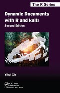
We can pass an argument width.cutoff to tidy_source() through the chunk option tidy.opts = list(width.cutoff = 40) so that the width of source code is roughly 40, e.g.,
Syntax highlighting comes by default in knitr (chunk option highlight = TRUE), since it enhances the readability of the source code — character strings, comments, and function names, etc., are in different colors. This is achieved by the highr package (Qiu and Xie, 2015). This option only works for ![]() and HTML output, and it is not necessary for Markdown because there are other libraries that can highlight code in Web pages; e.g., the JavaScript library highlight.js is widely used to do syntax highlighting for HTML pages.
and HTML output, and it is not necessary for Markdown because there are other libraries that can highlight code in Web pages; e.g., the JavaScript library highlight.js is widely used to do syntax highlighting for HTML pages.
For ![]() output, the
output, the ![]() package framed is used to decorate code chunks with a light gray background (as we can see in this book). If this package is not found in the system, a version will be copied directly from knitr. The output for HTML documents is styled with CSS, which looks similar to
package framed is used to decorate code chunks with a light gray background (as we can see in this book). If this package is not found in the system, a version will be copied directly from knitr. The output for HTML documents is styled with CSS, which looks similar to ![]() (with gray shadings and syntax highlighting). The background color is controlled by the chunk option
(with gray shadings and syntax highlighting). The background color is controlled by the chunk option background, which takes a color value such as ’#FF0000’, ’red’, or rgb(1, 0, 0) (as long as it is a valid color in R).
The prompt characters are removed by default because they mangle the R source code in the output and make it difficult to copy R code. The R output is masked in comments by default based on the same rationale (option comment = ’##’). In fact, this was largely motivated from the author’s experience of grading homework when he was a teaching assistant; with the default prompts, it is difficult to verify the results in the homework, because it is so inconvenient to copy the source code. Anyway, it is easy to revert to the output with prompts (set option prompt = TRUE), and we will quickly realize the inconvenience to the readers if they want to run the code in the output document, e.g., the chunk below uses prompt = TRUE and comment = NA:

While this may seem to be irrelevant to reproducible research, we would argue that it is of great importance to design styles that look appealing and helpful at first glance, which can encourage users to write reports in this way.
For ![]() output, we can also specify the font size of the chunk output via the size option, which takes the value of
output, we can also specify the font size of the chunk output via the size option, which takes the value of ![]() font sizes such as footnotesize, small, large, and Large, etc., (the default size is normalsize). It is helpful to set a smaller font size when the output is long and the space is limited, e.g., in beamer slides. The chunk below uses
font sizes such as footnotesize, small, large, and Large, etc., (the default size is normalsize). It is helpful to set a smaller font size when the output is long and the space is limited, e.g., in beamer slides. The chunk below uses size = ’footnotesize’:

We can show or hide different parts of the text output including the source code, normal text output, warnings, messages, errors, and the whole chunk. Below are the corresponding chunk options with default values in the braces:
echo (TRUE) whether to show the source code; it can also take a numeric vector like the eval option to select which expressions to show in the output, e.g., echo = 1:3 selects the first 3 expressions, and echo = −5 means do not show the 5th expression.
results (’markup’) how to wrap up the normal text output that would have been printed in the R console if we had run the code in R; the default value means to mark up the results in special environments such as ![]() environments or HTML
environments or HTML div tags; other possible values are:
’asis’ write the raw output from R to the output document without any markups, e.g., the source code cat (’<em>emphasize</em>’) can produce an italic text in HTML when results = ’asis’; this is very useful when we use R to produce raw elements for the output, e.g., tables using the ![]() markup (Section 6.3);
markup (Section 6.3);
’hold’ hold the text output and write to the end of the chunk;
’hide’ this option value hides the normal text output.
warning/error/message (TRUE) whether to show warnings, errors, and messages in the output; usually these three types of messages are produced by warning(), stop(), and message() in R.
split (FALSE) whether to redirect the chunk output to a separate file (the filename is determined by the chunk label); for ![]() ,
, input{} will be used if split = TRUE to input the chunk output from the file; for HTML, the <iframe> tag will be used; other output formats will ignore this option.
include (TRUE) whether to include the chunk output in the document; when it is FALSE, the whole chunk will be absent in the output, but the code chunk will still be evaluated unless eval = FALSE.
Below is an example that shows results = ’asis’ and three types of messages:


If we did not use the results option, we will see the raw ![]() code instead of an equation in the output:
code instead of an equation in the output:

As we have introduced in Section 5.1, we can use opts_chunk to set global chunk options. For instance, if we want to suppress all warnings and messages in the whole document, then we can do this in the first chunk of the document:
![]()
When warning = FALSE (or message = FALSE), warnings (or messages) will be printed in the R console instead of the report output. If you really want to suppress them, you have to call the function suppressWarnings() (or suppressMessages()) on the R expression, e.g.,

It may be very surprising to knitr users that knitr does not stop on errors! As we can see from the previous example, 1 + ’a’ should have stopped R because that is not a valid addition operation in R (a number + a string). The default behavior of knitr is to act as if the code were pasted into an R console: if you paste 1 + ’a’ to the R console, you will see an error message, but that does not halt R — you can continue to type or paste more code. To completely stop knitr when errors occur, we have to set the chunk option error = FALSE:
![]()
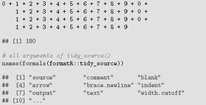
Currently this feature applies to R Markdown only. If a code chunk has many short R expressions, and each expression prints some output, it will be disturbing to read the output because R each expression and output fragment occupies a separate visual block. In this case, you can collapse all code and output fragments into one block using the chunk option collapse = TRUE. Here is an example:
This is what the default output looks like (i.e., when collapse = FALSE):

The chunk option strip.white (TRUE by default) can be used to strip blank lines at the beginning and end of a source code chunk. For example, the blank line at the end of this chunk will be removed by default:
![]()
Tables are essentially text output, but the first edition of this book did not cover table generation for a number of reasons:
1. this functionality is orthogonal to knitr — as long as we can find another package to create the table, knitr can easily show it in the output with the chunk option results = ’asis’; a few good examples include xtable (Dahl, 2014), Hmisc (Harrell, 2015), and tables (Murdoch, 2012);
2. it can be very challenging and complicated to generate tables for different document formats and different types of R objects, and the author has not found a perfect solution yet;
3. sometimes graphics can present the information better than tables, and it is much easier to make plots.
However, it seems there is still high demand on this particular feature, so we will expand this topic a little bit. For ![]() tables, the packages mentioned above should work well. For HTML tables, xtable and R2HTML (Lecoutre, 2014) can be used. Additionally, Table 1.1 is an example of kable(), a simple function provided in knitr for
tables, the packages mentioned above should work well. For HTML tables, xtable and R2HTML (Lecoutre, 2014) can be used. Additionally, Table 1.1 is an example of kable(), a simple function provided in knitr for ![]() , HTML, and Markdown tables. More importantly, the kable() function is aware of the output format, and can automatically generate a table of the appropriate format, e.g., for the same data object, it generates a
, HTML, and Markdown tables. More importantly, the kable() function is aware of the output format, and can automatically generate a table of the appropriate format, e.g., for the same data object, it generates a ![]() table in an Rnw document, a Markdown table in an Rmd document, and an HTML table in an R HTML document. Therefore, you do not need to remember which type of document you are in, and just call kable() in your code chunk. The code chunk below shows the source code of tables of different formats:
table in an Rnw document, a Markdown table in an Rmd document, and an HTML table in an R HTML document. Therefore, you do not need to remember which type of document you are in, and just call kable() in your code chunk. The code chunk below shows the source code of tables of different formats:


If you simply want to display rectangular data as plain tables, kable() can be a good choice. If you want more advanced and complicated features such as conditional formatting (e.g., color certain rows/cells), you are advised to use other packages.
Under the hood, knitr uses the S3 generic function knit_print() to print objects in R code chunks by default. All visible objects are passed to knit_print() to render text output. Basically, knit_print() is the same as print(), but you can extend this S3 generic function by writing S3 methods for it without changing R’s print() function. To know more details about this, please see the package vignette:
![]()
The printr package (Xie, 2014) has provided several S3 methods for the knit_print() function. Once this package is loaded, you can just type the object names in a code chunk, and knitr will know how to print them automatically according to the output format. For example, when you type ??sunflower in the R console (?? means help.search() in R), you will see a help window pop up showing the search results using the keyword “sunflower.” However, if you type this in an R code chunk, and compile it using knitr, normally you will see nothing because we cannot embed a transient help window in the output. Since ?? is essentially an R function that returns a special object of the class hsearch, the printr package has defined an S3 method knit_print.hsearch() to process the object of search results, so you can use the ?? command after loading the printr package:
![]()
Package |
Topic |
Title |
graphics |
sunflowerplot |
Produce a Sunflower Scatter Plot |
grDevices |
xyTable |
Multiplicities of (x,y) Points, e.g., … |
![]()
Sepal.Length |
Sepal.Width |
Petal.Length |
Petal.Width |
5.1 |
3.5 |
1.4 |
0.2 |
4.9 |
3.0 |
1.4 |
0.2 |
4.7 |
3.2 |
1.3 |
0.2 |
4.6 |
3.1 |
1.5 |
0.2 |
5.0 |
3.6 |
1.4 |
0.2 |
5.4 |
3.9 |
1.7 |
0.4 |
From the reader’s perspective, this is cleaner than an explicit call to table-generating functions such as kable() in code chunks: the reader does not need to know what the table function was behind the scenes, and perhaps does not care either.
In fact, you do not have to use the knit_print() function. It is just the default value for the chunk option render, which takes a printing function. You are free to define another printing function and assign it to the render option. As a trivial example, you can use render = print to restore to the default printing behavior in the R console (print() is a function in base R).
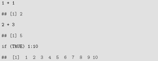
The syntax highlighting theme can be adjusted or completely customized. If the default theme is not satisfactory, we can use the object knit_theme to change it. There are about 80 themes shipped with knitr, and we can view their names by knit_theme$get(). Here are the first 20:
We can use knit_theme$set() to set the theme, e.g.,
![]()
Each theme contains a set of color and font definitions, which will be translated to ![]() commands or CSS definitions (for HTML) in the end. Note that syntax highlighting themes only work for
commands or CSS definitions (for HTML) in the end. Note that syntax highlighting themes only work for ![]() and HTML output. For Markdown, the highlight.js library also allows customization but that is beyond the scope of R and knitr. See
and HTML output. For Markdown, the highlight.js library also allows customization but that is beyond the scope of R and knitr. See http://bit.ly/knitr-themes for a preview of all these themes.
In the next chapter, we show how to control the graphics output.