Hooks are an important component to extend knitr. A hook is a user-defined R function to fulfill tasks beyond the default capability of knitr. There are two types of hooks: chunk hooks and output hooks. We have already introduced some built-in output hooks in Section 5.3, and how to customize both the chunk and inline R output. In this chapter we focus on chunk hooks.
A chunk hook is a function stored in knit_hooks and triggered by a custom chunk option. All chunk hooks have three arguments: before, options, and envir (explained later).
A chunk hook can be arbitrarily named, as long as it does not clash with existing hooks in knit_hooks. Names of all built-in hooks are:

For example, the name margin is not in the above names, so we can name a chunk hook as margin:


FIGURE 10.1: A plot with the default margin, i.e., par(mar = c(5.1, 4.1, 4.1, 2.1)).
This hook is used to set the margin parameter with par() for R base graphics (because the default margin is often too big).
After we have defined a hook, we need to set a chunk option with the same name to a non-NULL value in order to execute the hook function. By default all undefined chunk options are NULL, so the chunk below is equivalent to a chunk with the option margin = NULL, which will not call the hook we just defined when the chunk is compiled (Figure 10.1):

However, when we set margin = TRUE, the hook will be called before the chunk is evaluated because TRUE is not NULL (Figure 10.2):

We set the plot background to be gray just to show the margins more clearly.

FIGURE 10.2: A plot with a smaller margin using the margin hook (par(mar = c(4, 4, .1, .1))).
Now we explain the four arguments of a chunk hook. Note all four arguments are optional.
before a logical value: TRUE if the hook is called before a chunk, and FALSE when a hook is called after a chunk
options a list of current chunk options, e.g., options$label is the current chunk label
envir the environment in which the current code chunk is evaluated, e.g., envir$x is the object x in the current chunk (if it exists)
name the name of the current hook function
A chunk is called twice for a chunk: once before a chunk and once after a chunk. In the above margin hook, par() was called before a chunk is evaluated, so the plots will use the parameters set by par(). If we set par() after a chunk, it will be too late (hence useless) because the plots have already been drawn.
10.1.4 Hooks and Chunk Options
Since chunk hooks are called as long as the corresponding chunk options are not NULL, we can set these chunk options globally if we want the chunk hooks to be applied to all chunks in a document, e.g.,
![]()
Note that non-NULL does not necessarily mean TRUE; in the above example, we can also set margin = 1 or margin = ’hello’, and so on, because these values are not NULL either.
Since knitr accepts arbitrary chunk options, the options argument in chunk hooks can be very flexible. The previous example did not actually make good use of the chunk option margin, because this option was basically ignored in the hook. Now we extend the hook a little bit, with margin being a vector to be passed to par(mar = …):

Instead of using a fixed value c(4, 4, .1, .1) for the margin parameter, we can use any numeric vectors of length 4 now, e.g.,

Then before this chunk is evaluated, par(mar = c(2, 3, 1, .1)) will be called first.
Since a chunk hook is a function, it also has a returned value. If the value returned is character, it will be written to the output. The previous hooks did not write anything to the output because they did not return character values (par() returns a list).
Below is a hook that returns character values: a down brace ![]() before a chunk and an up brace
before a chunk and an up brace ![]() after a chunk.
after a chunk.

We apply this brace hook to the following chunk:

Chunk hooks that return character values allow us to write anything we want to the chunk output. One important application is to write images to the output, which we have created through R code in the chunk. The character values may be like includegraphics{…} (![]() ),
), <img src=’…’ /> (HTML) or  (Markdown), etc. This is the trick we will use for the next few sections, such as saving rgl and GGobi plots.
In this section we give some examples of chunk hooks, most of which have been predefined in knitr, i.e., we can use them directly after knitr has been loaded.
Some R users may have been suffering from the extra white margins in R plots, especially in base graphics (ggplot2 is usually better in this aspect). The default graphical option mar is about c(5, 4, 4, 2) as we mentioned in Figure 10.1 (also see ?par), which is often too big. Instead of endlessly tweaking par(mar), we may consider the program pdfcrop, which can crop the white margin automatically (http://www.ctan.org/pkg/pdfcrop). In knitr, we can set up the hook hook_pdfcrop() to work with a chunk option, say, crop.

FIGURE 10.3: The original plot produced in R, with a large white margin.
![]()
Now, we compare two plots produced by the same code chunk below. The first one is not cropped (Figure 10.3); then the same plot is produced but with a chunk option crop = TRUE, which will call the cropping hook (Figure 10.4).

As we can see, the white margins are gone (to better see the difference, we have put a frame box around each plot). If we use par(), it might be hard and tedious to figure out a reasonable amount of margin such that no label is cropped due to a too-small margin, nor do we get too large a margin.
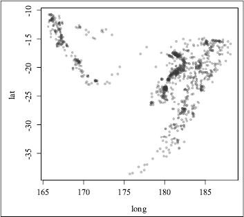
FIGURE 10.4: The cropped plot; obviously the white margins on the top and right have been removed.
With the hook hook_rgl(), we can easily save snapshots from the rgl package (Adler and Murdoch, 2014). The rgl hook is a good example of taking care of details by carefully using the options argument in the hook; for example, we cannot directly set the width and height of rgl plots in rgl.snapshot() or rgl.postscript(), so we make use of the options fig.width, fig.height, and dpi to calculate the expected size of the window, then resize the current window by par3d(), save the plot, and finally return a character string containing the appropriate code to insert the plot into the output. Here is a quick and dirty version of hook_rgl():


FIGURE 10.5: An rgl plot captured by hook_rgl(): this hook function calls rgl.snapshot() in rgl to save the snapshot into a PNG image.

The real hook function in knitr is much more complicated than this due to a lot of details to be taken into consideration. Below is an example of how to save rgl plots using the rgl hook. First we define a hook named rgl for the function hook_rgl():
![]()
Then we only have to set the chunk option rgl = TRUE and the captured plot is shown in Figure 10.5.

We have explained how R plots are recorded in Section 7.2. In some cases, it is not possible to capture plots by recordPlot() (such as rgl plots), but we can save them using other functions. To insert these plots into the output, we need to set up a hook first like this (see the help page ?hook_plot_custom for details):

FIGURE 10.6: A plot created and exported by GGobi, and written into ![]() by the hook hook_plot_custom().
by the hook hook_plot_custom().
![]()
Then we set the chunk option custom_plot = TRUE, and manually write plot files in the chunk. Here we show an example of capturing GGobi plots using the function ggobi_display_save_picture() in the rggobi package (Temple Lang et al., 2014):

Figure 10.6 is the plot output from GGobi. Two things to note here are:
1. we have to make sure the plot filename is from fig_path(), which is a convenience function to return the figure path for the current chunk (a combination of the chunk label, fig.path and fig.ext);
2. we need to set the chunk option fig.ext (figure file extension) because knitr will be unable to figure out its value automatically (we are not using any graphical devices).
We can even save a series of images to make an animation with the option fig.show = ’animate’ (Section 7.3.1); below is an example of zooming into a scatterplot using rgl (for the real animation, see knitr’s main manual):

The free software OptiPNG is a PNG optimizer that re-compresses image files to a smaller size, without losing any information (http://optipng.sourceforge.net/). In knitr, the hook function hook_optipng() is a wrapper around OptiPNG to compress PNG plots, and OptiPNG has to be installed beforehand; for Windows users, the executable has to be in the PATH variable. We can set up the hook as usual:
![]()
Then we can either set the chunk option optipng = TRUE to enable it for a chunk, or pass a character string to this option so that it is used by OptiPNG as additional command line arguments. For example, we can use optipng = ’-o7’ to specify the highest level of optimization. See the documentation of OptiPNG for all possible arguments.

FIGURE 10.7: Adding elements to an existing rgl plot: if we do not open a new device, latter elements will be added to the existing device.
The default rgl hook hook_rgl() does not close the rgl device before drawing a new plot, which may be problematic, because the latter plot is drawn on the previous scene. For example, we get one plot with two spheres (Figure 10.7) when we execute the following two lines together, but two plots with one sphere in each if we close the first plot and run the second line:
![]()
Normally different code chunks use different graphical devices, so graphical elements in a latter chunk will not be added to a previous chunk, but this is not true for rgl plots. In order to close the device before drawing plots, we have to tweak the hook a little bit, e.g.,

The function rgl.cur() returns the current device id; if it is greater than 0, it means there is an existing device, and we can close it by rgl.close().
We introduced how to save static rgl plots in Section 10.2.2. In fact, we can also export the rgl 3D plot into WebGL (http://en.wikipedia.org/wiki/WebGL) using the writeWebGL() function, so that the plot can be reproduced in a Web browser that supports WebGL. For example, we can rotate and zoom in/out the plot.
The hook function hook_webgl() in knitr is a wrapper to the WebGL function in rgl. With this hook, we can capture a 3D scene into the HTML output.