3	Membrane Channels and Action Potentials

This chapter continues our study of matrix models, but applies them to study molecular structures called membrane channels. The counterparts of different age classes of a population are different conformations of a channel. The transitions between age-classes for an individual and those between conformations for a channel are very different. Individuals never become younger, returning to a former age-class, while channels may revisit each conformation many times. Nonetheless, the theory of power-positive matrices is just the right tool for predicting the behavior of a large collection of channels, based on the behavior of individual channels.

Membrane channels are pores in the cell membrane that selectively allow ions to flow through the membrane. These ionic flows constitute electrical currents that are biologically important. This is especially apparent in electrical excitable tissue like skeletal muscles, the heart, and the nervous system. All of these tissues have action potentials, impulses of electrical current that affect ionic flows through membrane channels. Action potentials are a primary means of signaling within the nervous system. They are triggered by inputs to sensory neurons, communicate information among neurons throughout the nervous systems, and transmit motor commands to the musculoskeletal system. Action potentials coordinate the heartbeat, and malfunction of cardiac electrical activity is quickly fatal if proper function is not restored.

Dynamic models built upon extensive knowledge about the nervous system and other organs help us to understand action potentials and the electrical excitability of these complex systems. This chapter provides a brief overview of the electrical excitability of membranes at molecular and cellular levels. We use the mathematics of matrix algebra introduced in Chapter 2 to analyze models of how individual membrane channels function. There is also new mathematics here, namely, aspects of probability. The specific times that channels change their conformational states are unpredictable, so we introduce probabilistic models for these switching times. As in tossing a large number of coins, we can predict the average behavior of a large population of channels even though we cannot predict the behavior of individual channels. The measurements that can be made give us only partial information about the state of individual channels. Models and their analysis provide a means for “filling the gaps” and deducing information about things that cannot be observed directly.

We consider models at three different levels: a single ion channel, a population of channels of a single type, and multiple populations of several different channel types in a cell, whose interactions lead to the generation of action potentials. In each case, we review the biology underlying the models. The next level up—the patterns that can arise in a population of interconnected cells—is touched on in Chapter 7.

3.1 Membrane Currents

The membranes surrounding cells are for the most part impermeable, but they incorporate a variety of molecular complexes designed to transfer material across the membrane. The membrane allows cells to maintain different concentrations of ions inside the cells than outside. The imbalance of electric charge across the cell membrane creates an electrical potential difference. There are molecular complexes that use inputs of energy to maintain the concentration and electrical potential differences across the membrane. Membrane channels are different structures through which ions cross the membrane. Channels are pores that can open to allow ionic flows driven by diffusive and electrical forces (see Figure 3.1). You can imagine a channel as an electrical valve that allows ions to flow through when it is open and blocks ionic flows when it is closed. The electrical excitability of membranes relies on gating, the opening and closing of different types of channels. Channels have remarkable properties, notably:

• Many channels are selective, allowing significant flows only of particular ionic species. Channels that are specifically selective for sodium (Na⁺ ), potassium (K⁺ ), and calcium (Ca²⁺ ) ions are ubiquitous in the nervous system and important in the generation of action potentials.

• Channels have only a few distinct conformational states. Unlike a valve in a pipe that regulates the flow rate to any specified value up to a maximum, a channel only allows ions to flow at a rate determined by its conformational state and the driving forces. As we describe below, each channel state has a fixed conductance. The switching time between states is so rapid that we regard it as instantaneous. At fixed membrane potential, the current observed to flow has a small number of values, and the channel jumps abruptly from one to another.

Figure 3.1 Artist’s representation of a membrane-spanning channel with a diagram representing an equivalent electrical circuit for the channel (from Hille 2001, p. 17).

• Switching of channels among states appears to happen randomly. However, there are different probabilities for switching between each pair of states. These switching probabilities typically depend upon membrane potential (voltage dependence) or upon the binding of neurotransmitters to the membrane (ligand dependence).

Learning, memory, dexterity, and sensory perception are all mediated by the electrical signals within the nervous system. The “architecture” of this system is enormously complex, both at the cellular level and as a network of cells. For example, the human brain is estimated to have approximately 10¹² neurons. The geometry of most individual neurons is elaborately branched, with long processes called dendrites and axons. Pairs of neurons make contact at specialized structures called synapses, which can be either chemical or electrical. At chemical synapses, action potentials traveling along an axon of the presynaptic cell trigger the release of neurotransmitter into the intercellular space of the synapse. The neurotransmitter, in turn, binds to receptor sites on dendrites of the postsynaptic cell, stimulating a postsynaptic current.

Channels play a central role in the propagation of action potentials within neurons, along axons, and in synaptic transmission between nerve cells. Techniques for identifying the genes that code for channels and comparative studies of channels from different organisms are rapidly leading to catalogs of hundreds of different types of channels. Alternative splicing of these genes and modification of channels by events such as phosphorylation contribute additional diversity. Nonetheless, the basic structure and function of channels has been conserved throughout evolution. One place to start in understanding how the nervous system works is by considering an individual ion channel.

3.1.1 Channel Gating and Conformational States

The patch clamp recording technique invented by Neher and Sakmann (1976) makes it possible to measure the current through a single channel. A small piece of membrane is attached to a suction electrode and the current through this tiny patch of membrane is measured. If the patch is small enough, then it may contain a single channel and the measurements reflect the current flowing in that channel.

The first patch clamp studies were of the nicotinic acetylcholine receptors (nAChR) in the neuromuscular junction (Neher and Sakmann 1976). The recordings (Figure 3.2) exhibit the properties of channels listed above—in particular, the current switches between discrete levels at apparently random times. The nAChR receptor has two possible conductance levels, zero when it is closed and approximately 30 pS when open. From these recordings we obtain sequences of successive dwell times, the amounts of time that the channel remains open or closed before switching. These appear to be irregular, so we will turn to mathematical models that assume that the probability that the channel will switch states in a small interval depends on only its current state, and not its past history.

Biophysical models for channel gating are based upon the physical shape, or conformation, of the channels. Channel proteins can be modeled as a collection of balls and springs representing individual atoms and the forces between them. The springs correspond to covalent bonds, the strongest forces in the molecule. There are additional forces that depend upon the environment of the molecule and the three-dimensional shape of the molecule. Thermal fluctuations are always present, driving small energy changes through collisions and causing the molecule to vibrate. There is a free-energy function assigned to each spatial configuration of the atoms within the channel, and the physical position of the molecule is normally at states of smaller energy. The molecule spends relatively long periods of time near local minima of the free energy, undergoing only small vibrations. However, sometimes the thermal fluctuations are sufficiently large to cause the molecule to move from one local minimum to another.

The behavior of this system can be interpreted in terms of an “energy landscape.” Corresponding to any set of positions for the atoms is a value of the free energy, which we regard as defining a height at each point of this space. The resulting landscape has hills and valleys (see Figure 3.3). Imagine the state of the molecule as a particle vibrating on this landscape like a ball oscillating on a frictionless surface under the influence of gravity and being given small random kicks. The amplitude and frequency of vibrations of the particle around a minimum are determined by the steepness of the sides of the valley in the energy landscape. Occasionally, the molecule receives a kick that is hard enough to make it cross the ridge between one valley and another. The height of the ridge determines how frequently this occurs. When the molecule crosses to a new valley, it will settle at the new local minimum until it receives a kick that knocks it out of the valley surrounding that minimum. For any pair of local minima, there is a transition probability that the molecule will cross from the valley surrounding the first minimum to the valley surrounding the second. This transition probability depends only on the pair of states; in particular, it does not depend upon the past history of the particle. This leads to a model for the switching dynamics of the channel as a Markov chain, the type of mathematical model we study in the next section.

Figure 3.2 Data from a single channel recording of the nicotinic acetylcholine receptor (nAChR) channel in the neuromuscular junction, in the presence of four different agonists that can bind to the receptor. Note that the open channel current is the same for each agonist, but the dwell times are different (from Colquhoun and Sakmann 1985).

One important use of these models is to infer information about the conformational states of channels from measurements of membrane current. If each conformational state has a different conductance level, then the membrane current tells us directly about the conformational state. However, this is seldom true. Most channels have more than a single closed state, and some types of channel have multiple open states with the same conductance. The selectivity filter that determines the ion selectivity and permeability may be a small portion of the channel. Conformational changes that have little effect on this part of the channel are likely to have little effect on conductance.

Figure 3.3 A hypothetical energy landscape. Imagine a ball rolling along this curve under the influence of gravity and collisions with other, much smaller particles. When the ball sits at a local minimum, it stays near this minimum until it receives a “kick” hard enough to knock it over one of the adjacent local maxima.

To simplify matters, we shall only consider situations in which the channel conductance has just two values, one for open states and one for closed states. When we have only partial information about the molecular dynamics, we are left with the fundamental question as to whether we can model the dwell times of the channel from the information we do have. This is where mathematical analysis enters the picture.

Let us be careful here to specify in mathematical terms the problem that we want to solve. The channel that we want to model has conformational states C₁, C₂, . . . , C_k, O₁, . . . , O_l. The C_j are closed states and the O_j are open states. We do not know the numbers k and l of closed and open states: they are part of what we are trying to determine. The observations we make yield a time series of the membrane current at discrete times t₀, t₁, . . . , t_N. These measurements tell us whether the channel is in a closed state or an open state at each time. If the temporal resolution τ = t_i+1 − t_i is fine enough, then the probability of two or more transitions occurring in a single time step is very small. Assuming that this is the case, our data tell us when the channel makes transitions from an open state to a closed state, or vice versa. What information about the channel can we extract from these transition times? Can we determine values of k, l, and transition probabilities between states? How large are the expected uncertainties in our estimates associated with the limited amount of data that we have? What kinds of experiments can we do that will help us reconstruct more information about the switching process? These are the questions we shall examine more closely.

Exercise 3.1. Discuss how you expect the transition rates between two states to depend upon the height of the energy barrier between them. How do you think the distribution of amplitudes and frequency of the kicks affects the transition rates? Design a computer experiment to test your ideas.

3.2 Markov Chains

This section discusses the probability theory we use in models for membrane channels. Only in the next section do we return to the biology of channels.

Individual membrane channels are modeled as objects that have several conformational states, divided into two classes: open and closed. In open states, the channel allows a current flow of ions, while in closed states, it does not. If a channel has more than one open state, we assume that the current flow in each of the different open states is the same. We observe switching times between open and closed states of a channel, and then attempt to produce stochastic¹ models that reproduce the observed statistics of switching. Using simple examples of probability, we illustrate the principles and methods that lead to successful stochastic models of switching in some cases.

The stochastic models we discuss are Markov chains. Markov chain models are framed in terms of probabilities. We assume that a physical system has a finite number of states S₁, S₂, . . . , S_n, and that the system switches from one state to another at random times. The fundamental Markov assumption is that the switching probabilities depend only upon the current state of the system. Past history has no influence in determining the switching probability. Markov models can be formulated with either continuous time or discrete time. We shall emphasize discrete-time models in this chapter.

3.2.1 Coin Tossing

The simplest example of a Markov chain is a thought experiment of probability theory: flipping coins repeatedly. We think of a “fair” coin as having equal probability of landing heads or tails, but what does this mean since each toss must produce either heads or tails? The mathematical description of probability is built upon the idea of repetition of events. If we flip a coin once, there is no way to test the probabilities of the two different outcomes, heads and tails. From an experimental perspective, we view the probabilities as statements about the frequencies of these outcomes if we repeat an experiment many times. If we flip a coin N times, with N a large number, then we expect that a probability of 0.5 for each outcome will be reflected in roughly the same number of outcomes that are heads and outcomes that are tails. However, the exact numbers will fluctuate if we repeat the experiment of flipping a coin N times. Can we test whether observations are consistent with the hypothesis that a coin has equal probabilities of 0.5 for heads and tails by flipping it many times and observing the relative proportion of heads and tails? If the results for the series of experiments are highly improbable, then we reject them as being plausible. What we need here is a mathematical analysis of the probability distribution for sequences of N coin flips. This distribution is derived from the probabilities for an individual flip. In the mathematical idealization of the experiment of flipping a fair coin N times, all sequences of heads and tails of length N are equally likely outcomes and all are equally probable. By counting the number of sequences of length N with each number of heads and tails, we can assign probabilities to different outcomes that can be used in testing statistical hypotheses. Let us examine the case N = 4 to develop an intuition for the general case.

The possible outcomes of tossing the coin four times would be

where h represents the outcome of a head and t represents the outcome of a tail. Note that there are 2^N possible such sequences and so if the coin is fair, each of these sequences has equal probability, namely, 1/2⁴ = 1/16. Looking at the list, we count that there is 1 outcome with 0 heads, 4 outcomes with 1 head, 6 outcomes with 2 heads, 4 outcomes with 3 heads, and 1 outcome with 4 heads. Even though each (ordered) sequence of tosses is equally likely, it is six times more likely to observe 2 heads and 2 tails than to observe 4 heads. So we hypothesize that the probabilities of 0, 1, 2, 3, 4 heads are 1/16, 4/16, 6/16, 4/16, 1/16, respectively. Even though each sequence of tosses is equally likely, we expect to observe sequences with 2 heads and 2 tails about six times as often as we see sequences with 4 heads. If we perform a large number of sequences of four tosses and make a histogram for the number of trials with 0, 1, 2, 3, 4 heads, we expect that the bins of the histogram will have relative proportions close to 1/16, 4/16, 6/16, 4/16, 1/16.

The numbers 1, 4, 6, 4, 1 are the binomial coefficients that appear in expanding the polynomial

for k = 0, 1, 2, 3, 4. For the general case of sequences of N coin tosses, we use the expansion

where the c_k are the binomial coefficients

The distribution in the outcomes of flipping a fair coin N times is given by the binomial distribution defined by

This is justified by the following argument. There are 2^N possible outcomes for sequences of N coin tosses. If the coin is fair, then each of these sequences has equal probability, namely, 1/2^N. The number of sequences with k heads and N − k tails is given by the binomial coefficient c_k, so the probability of obtaining exactly k heads is b_k.

What happens if a coin is not fair? We want to compute the probabilities of different outcomes in a sequence of tosses of an unfair coin. Let H and T = 1 − H denote the probabilities of tossing a head or a tail, respectively. In the case of a fair coin, we have H = T = . The probability that a particular sequence of heads and tails occurs is given by the product of the corresponding probabilities. This is the assumption that the successive tosses are independent of each other. Thus the probability of the sequence hhth is HHTH. Placing subscripts on the H and T to denote the probabilities of the outcome of each toss, we write the formula

1 = (H₁ + T₁)(H₂ + T₂) . . . (H_N + T_N)

which expresses that either heads or tails is sure to be the outcome on each toss. Expanding the right-hand side of this formula, each of the 2^N sequences of heads and tails is represented by a single term that is the product of the probabilities of each outcome in that sequence of tosses. To determine the probability of all sequences with specified numbers of heads and tails, we drop the subscripts in the polynomial to get the formula

where the c_k are the binomial coefficients above. The number of sequences with exactly k heads is not affected by the probabilities of heads or tails, but the probability that a particular sequence of heads and tails with exactly k heads occurs is H^kT^N−k. Therefore, the probability of obtaining exactly k heads in a sequence of N independent tosses is c_kH^kT^N−k. To know what to expect when N is large, we compute and evaluate histograms of c_kH^kT^N−k.

It is convenient to plot these histograms with the horizontal axis scaled to be [0, l]: at k/N we plot the probability of having k heads in N tosses. Numerical computations with different values of H and N large suggest that the histograms are always approximated by a “bell shaped” curve with its peak at k/N = H (see Figure 3.4). This observation is confirmed by the DeMoivre-Laplace limit theorem, a special case of the central limit theorem of probability. This theorem states the following.

Consider a sequence of N independent coin tosses, each with probability H of obtaining heads. The probability of obtaining k heads with

approaches

as N → ∞.

The integrand in this formula is called the normal distribution. Other names for this important function are the Gaussian distribution and a bell-shaped curve. The DeMoivre-Laplace limit theorem tells us that in our coin-tossing experiment, as the length N of the sequence increases, the proportion k/N of heads is more and more likely to be close to H. The expected deviation of k/N from H is comparable to .

Diaconis, Holmes, and Montgomery (2004) reexamined the tossing of real coins and came to surprising conclusions. They built a coin-flipping machine and conducted experiments by repeatedly flipping a coin that starts heads up. The proportion of coin tosses in which the coin landed heads up was larger than l/2 by an amount that was statistically significant. In other words, if one assumes that the probability of landing heads was 1/2 and that the tosses were independent of each other, then the DeMoivre-Laplace theorem implies that the results they observed were very unlikely to have occurred. They went further with a careful examination of the physics of coin tossing. They found that reasonable hypotheses lead to the conclusion that it is more probable that a coin lands with the same side up that was face up at the beginning of the toss. Here we rely on computer experiments, using algorithms that generate pseudorandom numbers— sequences of numbers that look as if they are independent choices from a uniform probability distribution on the interval [0,1] (Knuth 1981). There are different approaches to the generation of pseudorandom numbers, and some widely used generators produce poor results.

Figure 3.4 A histogram from a computer experiment: 5000 repetitions of tossing an unfair coin 100 times. The probability of heads is 0.75 and the probability of tails is 0.25. The asterisks show the number of experiments that produced k heads as a function of k, the circles are the values of the binomial distribution, and the solid line is the approximation to the binomial distribution from the bell shaped Gaussian function. Note that the minimal number of heads obtained in our trials was 60 and the maximum was 91. There are small deviations from the predicted distribution that change when we rerun the experiment with different sequences of the random numbers used to generate the experimental outcome.

Exercise 3.2. Consider a sequence of 100 tosses of a fair coin. Use the DeMoivre-Laplace limit theorem to check the following statements. The odds (probability) of obtaining fewer than 20 heads is less than one in a billion. The odds of obtaining fewer than 30 heads is about one in 25,000, and the odds of obtaining fewer than 40 heads is less than three in 100. The odds of obtaining between 40 and 60 heads is more than 94 in 100, but there is more than a 5% chance of obtaining fewer than 41 or more than 59 heads. If one tosses a coin 10,000 times, there is more than a 95% chance of obtaining between 4900 and 5100 heads.

Exercise 3.3. Experiment with sequences of coin flips produced by a random number generator:

(a) Generate a sequence r of 1000 random numbers uniformly distributed in the unit interval [0, 1].

(b) Compute a histogram for the values with ten equal bins of length 0.1. How much variation is there in values of the histogram? Does the histogram make you suspicious that the numbers are not independent and uniformly distributed random numbers?

(c) Now compute sequences of 10,000 and 100,000 random numbers uniformly distributed in the unit interval [0, 1] and a histogram for each with ten equal bins. Are your results consistent with the prediction of the central limit theorem that the range of variation between bins in the histogram is proportional to the square root of the sequence length?

Exercise 3.4.

(a) Convert the sequence of 1000 random numbers r from the previous exercise into a sequence of outcomes of coin tosses in which the probability of heads is 0.6 and the probability of tails is 0.4.

(b) Recall that this coin-tossing experiment can be modeled by the binomial distribution: the probability of k heads in the sequence is given by

       c_k(0.6)^k(0.4)^1000−k

where c_k = 1000!/k!(1000 − k)!. Calculate the the probability of k heads for values of k between 500 and 700 in a sequence of 1000 independent tosses. Plot your results with k on the x-axis and the probability of k heads on the y-axis. Comment on the shape of the plot.

(c) Now test the binomial distribution by doing 1000 repetitions of the sequence of 1000 coin tosses and plot a histogram of the number of heads obtained in each repetition. Compare the results with the predictions from the binomial distribution.

(d) Repeat this experiment with 10,000 repetitions of 100 coin tosses. Comment on the differences you observe between this histogram and the histogram for 1000 repetitions of tosses of 1000 coins.

3.2.2 Markov Chains

A small generalization of the coin-flipping experiment produces a two-state Markov chain. In this generalization, one has two coins, each with its own heads versus tails probabilities. We will call one coin a penny and the other a quarter. The two possible states are that we are flipping either a penny or a quarter at each turn. We switch states according to the following:

• After a heads, we flip the penny

• After a tails, we flip the quarter

Given states S₁ and S₂, which may be the same, we call the transition probability from S₁ to S₂ the probability that we are in state S₁ at time t and in state S₂ at time t + 1. In the example, there are four transition probabilities associated with the current state and the outcome of the flip we do now. Since the coin we toss depends on the previous outcome, the transition probabilities are the probabilities of heads previous and heads now, heads previous and tails now, tails previous and heads now, and tails previous and tails now. These can be written in a 2 × 2 matrix called the transition matrix of the Markov chain.

Let us pick specific probabilities for the two coins to make our discussion more concrete. Assume that the probability of getting heads when we toss the penny is 0.4 and so the probability of getting tails is 1 − 0.4 = 0.6, and that the probability of getting heads when we toss the quarter is 0.7 and so the probability of getting tails is 1 − 0.7 = 0.3. Then the transition matrix for this system is

This means that if we are currently flipping the penny, then the probability that next time we will flip a penny is 0.4 and the probability that next time we will flip a quarter is 0.6. If we are currently flipping a quarter, the probability that next time we will flip a penny is 0.7 and the probability that next time we will flip a quarter is 0.3.

The behavior of the Markov chain can be different from flipping a single coin. For example, if the probability of flipping heads for the penny and the probability of flipping tails for the quarter are both less than 0.5 as in the example above, then we expect a larger number of alternating strings of penny:tails, quarter:heads than of successive quarter:heads or successive penny:tails. Repeated runs of heads and tails are less frequent than when flipping a single coin. On the other hand, if the probability of flipping tails for the penny is very low and the probability of flipping heads for the quarter is very low, then we expect a large number of repeated runs of both heads and tails. When the probabilities of heads and tails are independent of the current state, that does not happen. In that case, only one outcome can have high probability since the sum of the probabilities is 1. Runs of the outcome with low probability are very rare. The lengths of runs are directly relevant to our observations of membrane channels: if one thinks of the states of the Markov chain as being open and closed states of a membrane channel, the lengths of “runs” of the Markov chain correspond to the dwell times of the channel in open or closed states.

A Markov chain model can be represented by its transition matrix: the n × n matrix A is defined by setting the entry A_ij to be the probability that state S_j switches to state S_i. The sum of the entries in each column of A adds to 1 since state S_j surely switches to some state S_i at each time-step. This way of looking at the Markov chain allows us to relate its properties to those of matrix population models. We compare the states of the Markov chain with stages of a population, and the transition matrix of the Markov chain with the transition matrix of the population. We imagine a large population of individuals distributed among the states of the Markov chain. Each individual independently makes a transition to a new state using the probabilities in the transition matrix. The sample paths of the Markov chain are paths taken by individuals, and the transition matrix coefficient A_ij approximates the proportion of individuals in state S_j at time t who move to state S_i at time t + 1.

The matrix makes it easy to compute the transition probabilities for paths of length longer than 2. Consider the transition from state S_k to S_j to S_i in two steps. The Markov assumption implies that the probability for the two transitions to take place at successive time-steps is the product A_ijA_jk. Also, the probability that state S_k will make a transition to state S_i in two steps is

the (i, k) component of the matrix product of A with itself. Extending this argument, the probability that a sequence of length l beginning at state S_j ends at state S_i is (A^l)_ij, the (i, j) component of the matrix product A^l of A with itself l times.

The matrix A has non-negative entries. If it is power-positive, then we can use the Perron-Frobenius theorem to tell us about the evolution of our population: it will have a dominant eigenvalue and the eigenvector of the dominant eigenvalue is the only eigenvector with all positive entries. Since the sum of each column of A is 1, the row vector (1, 1, . . . , 1) is a left eigenvector with eigenvalue 1. Intuitively, growth rate 1 makes sense since our population is being redistributed among the states with no births or deaths in the population. Thus, the total population size remains constant. In formulas, if (w₁, w₂, . . . , w_j) is the population vector at time t, then the population vector at time t + 1 is

and the total population is

unchanged from time t. The Perron-Frobenius theorem implies that the population distribution will converge to the stable stage distribution, the right eigenvector of 1 for the transition matrix A. In the setting of membrane channels, there is an actual population of individual channels and the stable stage distribution gives the expected number of channels in each state under steady-state conditions. Moreover, the conductance of the membrane is the conductance of a single channel times the number of open channels.

Single-channel recordings of membrane currents show us transitions between open and closed states. Therefore, we are particularly interested in the residence or dwell times of a Markov chain, the times that a sample path remains in a particular state. In the channel, these transitions are the result of stochastic fluctuations and we assume that the time between measurements is short enough that the probability of multiple transitions between successive measurements is negligible. When the time-step is small enough, during most time-steps a channel remains in the same state. This implies that the transition matrix has diagonal entries A_jj close to 1 and the remaining entries are small.

We seek to determine the distribution of residence times for each state. If a channel is in state S_j at time t₀, the probability that it remains in state S_j at time t₀ + 1 is A_jj. The probability that it remains in the state S_j at times t₀ + 1 and . Continuing, the probability that the channel remains in state S_j for times . Similarly, the probability that the system switches from state S_j to some other state at each time is 1 – A_jj. The channel has a residence time of k in state S_j beginning at time t₀ if it is in state S_j at times t₀ < t < t₀ + k and it switches to another state in the step from time t₀ + k – 1 to t₀ + k. The probability associated with this sequence of states is . We conclude that the residence times have an exponential distribution: the probability of residence time k in state S_j decreases exponentially with k. If the time between measurements is δ and A_jj = exp(–λ_jδ), then the probability that a channel in state S_j makes its first transition to another state between times kδ and (k + 1)δ is (1 − A_jj) exp(−kλ_jδ).²

These results yield predictive information that we can utilize in analyzing the data from single-channel patch clamp measurements of membrane current. In the situation where we measure just two current levels (from open and closed states of the channel), our analysis of residence times predicts that histograms of the residence times will be sums of exponentials, with one exponential term for each channel state. Given time series data from a single-channel recording, we construct a histogram for the residence times of open states and the residence times of closed states. If there is a single open state, then the residence time histogram for the open state can be fitted by a single exponential function. If we need to sum more than one exponential to fit the histogram, then there must be more than one open state. The same conclusions apply to closed states. The number of exponential functions we need to fit the residence time histogram of the closed states gives a lower bound on the number of closed states of the channel.

Exercise 3.5. The histogram of expected residence times for each state in a Markov chain is exponential, with different exponentials for different states. To observe this in the simplest case, use a random number generator to produce data for a two-state Markov chain. Next, determine the transitions that occur in these data as the state changes, and the residence times between these. Finally, compute histograms of the residence times.

3.2.3 The Neuromuscular Junction

Using the theory that we have developed for Markov chain models, we now want to use single-channel patch clamp recordings to infer properties of the molecular mechanisms underlying the gating (opening and closing) of nAChR channels at the neuromuscular junction. Since the only step in this multistep process that is observed directly in these recordings is the final opening of the channel, analysis of the dwell times is required to deduce information about the steps taking place while the channel is closed.

The simplest possible model is that receptors with bound acetylcholine agonist are open, while unbound receptors are closed. The total membrane current would then be perfectly correlated with the amount of bound acetylcholine. This model is much too simple to explain two important observations. First, at low agonist concentrations, the current from a population of channels is seen to be roughly proportional to the square of agonist concentration rather than linearly proportional (Katz and Thesleff 1957). This cooperativity suggests that enhancement of the opening probability of a channel depends on a pair of agonist molecules binding to a channel, rather than a single bound molecule. Second, the dwell time distributions have “bursts” typified by several successive very short closings interspersed with long ones (Colquhoun and Sakmann 1985). This distribution of dwell times is not well approximated by a single exponential, implying that a Markov model for a single channel must have two or more closed states.

Colquhoun and Sakmann (1985) studied the dwell time distributions of open and closed states for the nAChR channels and how these vary with different experimental conditions. They varied membrane potential, agonist concentration, and the agonist itself. Acetylcholine is not the only molecule that binds to the receptors and acts as an agonist for the receptors, so use of different agonists is a way of exploring the dynamics of binding. Figure 3.2 shows recordings of single-channel recordings from their paper. They found in these studies that a sum of at least three exponentials was required to fit the dwell time distributions for closed states and a sum of at least two exponentials was required to fit the dwell time distributions for open states (see Figure 3.5). They postulated that the closed states are receptors with 0, 1, and 2 agonists bound, and that the open states have 1 or 2 agonists bound. Of special note here is that the transitions between open and closed states are distinct from the binding events of the agonist. Agonist binding changes the probability that a channel will open, but the binding itself does not open the channel. Figure 3.6 shows a diagram of the five-state model proposed by Colquhoun and Sakmann. The transition matrix for a Markov model corresponding to this graphical representation of the model has the approximate form I + δA for small time steps δ, where A is the following matrix expressing the rates of transitions between pairs of states.³

Figure 3.5 Sums of exponentials fit to dwell time distributions of open states in an nAChR channel. The three histograms show distributions of dwell times from three ranges of times: slow (top), medium (middle), and fast (bottom). The dashed curves come from a fit to a sum of two exponentials, the solid curves from a fit to a sum of three exponentials (from Colquhoun and Sakmann 1985).

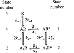
Figure 3.6 A diagram of the states and transitions in the Markov chain model used to model the nAChR channel (from Colquhoun and Sakmann 1985). The states labeled with an * are the open states.

with x_A the agonist concentration. The diagonal term A_jj of A gives the rate of decrease of channels in state j which remain in state j. Since the total number of channels does not change, the magnitude of this rate is the sum of the rates with which channels in state j make a transition to some other state. Colquhoun and Sakmann (1985) discuss parameter fits to this model from the dwell time distributions for different agonists. They find a good fit to the dwell times for acetylcholine by ignoring the state with a singly bound opening (AR* in the diagram) and the remaining parameters set to k₋₁ = k₋₂ = 8150 s⁻¹, k₊₁ = k₊₂ = 10⁸ s⁻¹(M)⁻¹, α = 714, and β = 30, 600.

Exercise 3.6. This exercise examines Markov chains with three states: one “open” state O and two “closed” states C₁ and C₂. We assume that measurements do not distinguish between the states C₁ and C₂, but we want to demonstrate that there are more than two states.

(a) Generate a set of 1,000,000 samples from the Markov chain with transition matrix

You can see from this matrix that the probability 0.7 of staying in state C₂ is much smaller than the probability 0.98 of staying in state C₁ or the probability 0.95 of remaining in state O.

(b) Compute the eigenvalues and eigenvectors of the matrix A. Compute the total time that your sample data in the vector states spends in each state and compare the results with predictions coming from the dominant right eigenvector of A.

(c) Produce a new vector rstates by “reducing” the data in the vector states so that states 1 and 2 are indistinguishable. The states of rstates will be called “closed” and “open.”

(d) Plot histograms of the residence times of the open and closed states in rstates.

(e) Comment on the shapes of the distributions for open and closed states. Show that the residence time distribution of the closed states is not fitted well by an exponential distribution. Using your knowledge of the transition matrix A, make a prediction about what the residence time distributions of the open states should be.

The nAChR channel illustrates the complexity of gating of membrane channels. Measurements of unitary currents through individual channels are conceptually simple, but the behavior of the channel is not. Abstract Markov chain models help answer questions about a complex multistep process without incorporating detail about the physics of binding or gating. Our discussion has brought forward basic principles about how these stochastic models are fit to the data, but we have just touched the surface of these principles are applied. Here are three mathematical questions arising from the limitations of the experimental techniques. They give pointers to how the analysis becomes more complicated.

1. The instrumental noise in patch clamp current measurements may be comparable to the current flowing through an open channel. How do we distinguish the times when the channel is truly open and truly closed?

2. If a channel opens and closes between two successive measurements, we do not observe these transitions. What effect do such short visits to a closed or open state have on our estimates?

3. We assume that there is a single channel in the patch of membrane in our apparatus. How do we tell? If we see the combined current from two open channels simultaneously, this is clear evidence for multiple channels in the patch. However, if openings are short and infrequent, we may have to watch for a long time before two channels are open simultaneously. How long is long enough to make us confident that we have a single channel?

These questions are discussed by Colquhoun and Hawkes (1995).

3.3 Voltage-Gated Channels

We now move up a level—from models of a single channel to models for a population of channels that are voltage gated, meaning that their transition probabilities between conformational states are a function of the potential difference across the membrane. The statistical summation of all ion currents from the channels in a patch of membrane behaves in a much more predictable fashion than the instantaneous on/off current through a single channel. The central limit theorem of probability theory predicts that the relative magnitude of the fluctuations in the current will be comparable to the square root of the number of channels contributing to the current. Since the total current is proportional to the number of channels, the relative magnitude of the fluctuations decreases as the population size grows.

What are the quantitative relations between the ionic current flowing through a population of channels, the fluctuations in this current, the unitary current through an individual channel, and the population size? This is the question we now explore using the probability theory in section 3.2. To begin, we make several assumptions about the channels and the membrane in which they are embedded:

• The voltage potential across the membrane is held constant (this experimental manipulation is called a voltage clamp, and the experimental methodology to achieve it was first developed by Hodgkin and Huxley (1952)).

• There are N channels in a membrane randomly switching between open and closed states.

• The current through each open channel is the same.

• The state of each channel is independent of the others.

These assumptions lead to similarities with the coin-tossing problem. Let the probability that a single channel is open be p and the probability that it is closed be q = 1 − p. At each time, we can represent the state of the system as a vector (a₁, . . . , a_N) where each a_i is a C for closed or O for open. There are 2^N different sequences representing the possible states of the system at each time. The assumption that the states of the individual channels are independent means that the probabilities of the population being in a given state is the product of the probabilities for the individual channels: if there are k open channels and N − k closed channels, the probability of the state (a₁,. . . , a_N) is p^k(1 − p)^(N−k). Using the same combinatorics as in coin tossing, the probability that there are exactly k open channels at each time is

Even though analysis of dwell times may require a complicated Markov model with multiple states of each channel, independence implies that the current flow in the population has a binomial distribution. If we sample the population at times that are long compared to the switching time of the individual channels, then the samples will be independent of each other. This provides helpful information that relates the population current, the individual channel current, and the fluctuations in the channel current. We derive below a formula for this relationship.

Let the current of a single open channel in our population be i. This depends on the membrane potential, but that is held constant in voltage clamp. If k channels in the population are open, then the population current is ki. The DeMoivre-Laplace Limit Theorem stated earlier tells us that as N grows large, the expected value of k is pN with fluctuations in k of magnitude proportional to An alternative calculation works directly with the population current measurements. When we measure the current in a population of N channels repeatedly, is expected to be the mean population current. Think of this current as the analog of tossing N coins simultaneously, with p the probability of heads for each. Measuring the population currents M times, obtaining values I_j, we expect the average population current

to be closer to the mean than the typical I_j. Fluctuations in the measurements of the population current can be measured by the variance σ, defined by the formula

Expanding the term for in this formula and a bit of algebra give the alternative formula

for σ. These population level measurements of mean and variance can be related to those for a single channel by the following argument.

If we measure current from a single channel M times, then we expect that the channel will be open approximately k = pM times, so the mean current from individual channels will be pi = (1/M)ki. If k of the individual channels are open, the variance of the single-channel measurements is

Now, if each of our population of N channels behaves in this manner, the mean current will be I = Npi and the variance will be obtained from adding the variances of the individual channels in the equation [3.1] for σ²:

We eliminate N from this last formula using the expression N = I/(pi) to obtain σ² = iI − piI and then solve for i:

This is the result that we are after. It relates the single-channel current to the population current and its variance. The term (1 − p) in this expression is not measured, but it may be possible to make it close to 1 by choosing a voltage clamp potential with most of the channels in the population closed at any given time.

Fluctuation analysis based upon this argument preceded the development of single-channel recordings based upon patch clamp. Thus, one can view the formula for the single-channel current as the basis for predictions of the unitary conductance of single channels. This analysis was carried out by Anderson and Stevens (1973) on the nAChR channel, giving an estimate of 30 pS for the unitary conductance. Subsequent direct measurements with patch clamp gave similar values, in accord with the theoretical predictions. Thus, the theory of coin tossing applied to the fluctuations in total current from a population of membrane channels gave successful predictions about the number of individual channels and their conductances. This was science at its best: data plus models plus theory led to predictions that were confirmed by new experiments that directly tested the predictions.

3.4 Membranes as Electrical Circuits

We now go up one more level, to consider the interactions among several different types of voltage-gated channels in a single neuron, and the patterns of neural activity that can result, such as action potentials. The interaction between voltage-gated channels is indirect, mediated by changes in the electrical potential (voltage difference) across the membrane. As ions flow through channels this changes the electrical potential across the membrane, which in turn changes the transition probabilities for all voltage-gated channels. In the last section, we saw that the relative magnitude of the fluctuations in a population of identical channels tends to 0 as the size of the population increases. In other words, large populations of thoroughly random individual channels behave like deterministic entities, so we model them that way. Models at this level are based on regarding the membrane and its channels as an electrical circuit—such as that depicted in Figure 3.1—so it is helpful to begin by reviewing a few concepts about circuits.

Electric charge is a fundamental property of matter: electrons and protons carry charges of equal magnitude, but opposite sign. Electrons have a negative charge, protons a positive charge. Charge adds: the charge of a composite particle is the sum of the charges of its components. If its charges do not sum to zero, a particle is an ion.

Charged particles establish an electric field that exerts forces on other charged particles. There is an electromotive force of attraction between particles of opposite electric charge and a force of repulsion between particles of the same charge. The electric field has a potential. This is a scalar function of position whose gradient⁴ is the electric field. The movement of charges creates an electrical current. Resistivity is a material property that characterizes the amount of current that flows along an electrical field of unit strength. Resistance is the corresponding bulk property of a substance. The resistance of a slab of material is proportional to its resistivity and thickness, and inversely proportional to its surface area. Conductance is the reciprocal of resistance, denoted by g_K in Figure 3.1.

Channels in a membrane behave like resistors. When they are open, channels permit a flow of ions across the membrane at a rate proportional to v − v_r where v is the membrane potential and v_r is the reversal potential discussed below. The membrane potential relative to v_r makes the membrane act like a battery, providing an electrodiffusive force to drive ions through the channel. This potential is labeled E_K in Figure 3.1. Even though membranes are impermeable, an electric potential across them will draw ions of opposite polarity to opposite sides of the membrane. The accumulation of ions at the membrane surface makes it an electrical capacitor (with capacitance C_M in Figure 3.1). The movement of these electrical charges toward or away from the membrane generates a current, the capacitive current CdV/dt, despite the fact that no charge flows across the membrane. Charge movement is induced by changes in the membrane potential, proportional to the change in the membrane potential. This leads to Kirchhoff’s current law, the fundamental equation describing the current that flows between the two sides of the membrane:

In [3.2], C is the membrane capacitance and each term g_j(v − v_j) represents the current flowing through all the channels of type j. Here v_j is the reversal potential of the channels of type j and g_j is their conductance. For voltage-gated channels, g_j itself changes in a way that is determined by differential equations. This aspect of channel behavior will be investigated later in Section 3.4.2.

Exercise 3.7. Using electrodes inserted into a cell, it is possible to “inject” current into a cell, so that [3.2] becomes

A “leak” current is one with constant conductance g_L. Show that changes in the reversal potential v_L of the leak current and changes in l_i, the injected current, have similar effects on the membrane current. Discuss the quantitative relationship between these.

3.4.1 Reversal Potential

The ionic flows through an open channel are affected by diffusive forces as well as the electrical potential across the membrane. Membrane pumps and exchangers can establish concentration differences of ions inside and outside a neuron. They rely upon active shape changes of the transporter molecules and inputs of energy rather than diffusive flow of ions through the pores of membranes. Pumps and exchangers operate more slowly as ion transporters than channels, but they can maintain large concentration differences between the interior and exterior of a cell. In particular, the concentration of K⁺ is higher inside the cell than outside, while the concentrations of Na⁺ and Ca²⁺ ions are higher outside.

Diffusive forces result from the thermal motions of molecules. In a fluid, particles are subject to random collisions that propel them along erratic paths called Brownian motion. The resulting diffusion acts to homogenize concentrations within the fluid. Near a channel, the intracellular and extracellular spaces are maintained at different concentrations, so the concentration within the channel cannot be constant: there must be a concentration gradient. At equilibrium and in the absence of other forces, the concentration of an ion in a tube connected to two reservoirs at differing concentrations will vary linearly, and there will be a constant flux of ions flowing from the region of high concentration to the region of low concentration.

The electrical force across a membrane is proportional to its potential. This electrical force may be directed in the same direction as the diffusive forces or in the opposite direction. The diffusive and electrical forces combine to determine the motion of ions in an open channel. As the membrane potential varies, there will be a specific potential, the reversal potential, at which the two forces balance and there is no net flux of ions. At higher potentials, the net flow of ions is from the interior of the neuron to the exterior. At lower potentials, the ionic flux is from the exterior to the interior. The Nernst equation gives a formula for the reversal potential through a channel selective for a single species of ions: the reversal potential is proportional to ln(c₁/c₂) where c₁ is the external concentration and c₂ is the internal concentration.

Even though the ionic flow through channels is faster than the transport of ions by the pumps and exchangers, it is small enough that it has a minimal effect on the relative internal and external concentrations of K⁺ and Na⁺ ions. Ca²⁺ ions play essential roles as signaling molecules, and large increases in local concentrations of Ca²⁺ ions due to the influx through calcium channels have important effects on electrical excitability in some cases. Accordingly, internal calcium ion concentration is used as a variable in many models of membrane excitability, but the concentrations of sodium and potassium are constant in virtually all models. The dynamics of calcium concentration within cells is an active area of intense research, aided by the ability to visualize calcium concentrations with special dyes.

Exercise 3.8. The full expression for the reversal potential in the Nernst equation is

where R is the gas constant 1.98 cal/K-mol, F is the Faraday constant 96, 840 C/mol, T is the temperature in K, and z is the valence of the ion. The value of RT/F is approximately 26.9 mV at T = 37° C = 310 K. Typical values of c₁ and c₂ for sodium ions in a mammalian cell are 145 and 15 mM. Compute the reversal potential for sodium in these cells.

3.4.2 Action Potentials

We now return to considering the total current flowing through all the channels in a membrane. Typical neurons and other excitable cells have several different types of voltage-gated channels whose currents influence one another. In our representation of the membrane as a circuit, each type of channel is represented by a resistor. Current through each type of channel contributes to changing the membrane potential, and the conductance of the channel is voltage dependent. Quantitative models are needed to predict the effects of this cycle of interactions in which current affects potential which affects current. As the number of channels of each type in a membrane increases, the relative magnitude of the fluctuations in the population current decrease. In many systems, the relative fluctuations are small enough that we turn to deterministic models that represent the total current of populations of voltage gated channels explicitly as a function of membrane potential. This leads to a class of models first proposed by Hodgkin and Huxley (1952) to model action potentials.

The primary object of study in the Hodgkin-Huxley model is the time-dependent membrane potential difference v(t). We assume a “space clamped” experimental setup in which the potential difference is uniform across the membrane, so spatial variables are not included in the model. The potential difference results from ionic charges on the opposite sides of the membrane. The membrane itself acts like a capacitor with capacity C. The specific capacitance (capacitance per unit area) is usually given a nominal value of 1 μF/cm². Membrane channels act like voltage-dependent resistors, and support current flowing through the membrane.

The first ingredient in the Hodgkin-Huxley model is simply Kirchhoff’s law, [3.2], which says that Cdv/dt is given by the sum of currents flowing through the membrane channels. However, to complete the model we also have to specify how the changes in potential affect the conductances g for each type of channel. The remainder of this section describes the formulation of models using the approach established by Hodgkin and Huxley. The mathematical and computational methods used to derive predictions from these models are discussed in Chapter 5.

Hodgkin and Huxley observed two distinct types of voltage-dependent membrane currents: one permeable to potassium ions and one permeable to sodium ions. There is a third type of channel, called the “leak,” with conductance that is not voltage dependent. Channels had not been discovered when they did their research. One of their contributions was the development of “voltage clamp” protocols to measure the separate conductances and their voltage dependence.

To fit their data for the sodium and potassium currents, they introduced the concept of gating variables, time-dependent factors that modulated the conductance of the currents. Today, these gating variables are associated with the probabilities of channel opening and closing.

In the Hodgkin-Huxley model, there are three gating variables. The gating variables m and h represent activation and inactivation processes of the sodium channels while the gating variable n represents activation of the potassium channels. The gating variables themselves obey differential equations that Hodgkin and Huxley based on experimental data. Figure 3.7 shows a set of current traces from voltage clamp measurements of the squid axon.

To understand the kinetics of channel gating, a few more facts and a bit more terminology are needed. As in all electrical circuits, membrane potential has an arbitrary baseline. The convention in neuroscience is to set the potential outside the membrane to be 0 and measure potential as inside potential relative to the outside. The resting potential of most neurons, as well as the squid giant axon, is negative and in the range of −50 to −80 mV. If the membrane potential is made more negative, the membrane is said to be hyperpolarized. If the potential is made more positive, the membrane is depolarized. Processes that tend to increase the probability of a channel opening with depolarization are called activation processes. Processes that tend to decrease the probability of a channel opening with depolarization are called inactivation processes. The reversal of of an activation process with hyperpolarization is called deactivation and the reversal of an inactivation process with depolarization is called deinactivation.

Figure 3.7 Data from a series of voltage clamp measurements on a squid giant axon. The membrane is held at a potential of −60 mV and then stepped to higher potentials. The traces show the current that flows in response to the voltage steps (from Hille 2001, p. 38).

Deactivation and inactivation are very different from one another, but both processes can act on the same channel. The Hodgkin-Huxley model assumes that the activation and inactivation processes of the sodium channels are independent of each other. Imagine there being two physical gates, an activation gate and an inactivation gate, that must be open for the channel to be open. As the membrane depolarizes, the activation gate is open more of the time and the inactivation gate is closed more. Deactivation reflects the greater tendency of activation gates to close with hyperpolarization. The Hodgkin-Huxley model also assumes that the gating of each type of channel depends only on the membrane potential and not upon the state of other channels.

The kinetics of activation and inactivation processes are not instantaneous, so the gating variables are not simple functions of membrane potential. To study these kinetics, Hodgkin and Huxley used voltage clamp protocols. Instead of measuring the membrane potential, they measured the current in a feedback circuit that maintained the membrane at a fixed, predetermined potential. Under these conditions, the gating variables approach steady-state values that are functions of the membrane potential. One of the fundamental observations leading to the models is that the currents generated as the membrane approaches its steady state can be modeled by sums of exponential functions. In a similar fashion to the analysis of residence times in Markov chain models, this suggests that, at any fixed membrane potential, the gating variables should satisfy linear differential equations.

Recall that exponential functions are solutions of linear differential equations. The differential equations describing the gating variables are frequently written in the form

where τ and x_∞ are functions of the membrane potential. The solution of this equation is

This formula expresses quantitatively the exponential relaxation of the variable x to its steady state (or “infinity”) value x_∞ with the time constant τ. The Hodgkin-Huxley model has equations of this form for each of the gating variables m, n, h. For each gating variable, the voltage-dependent steady-state values and time constants are measured with voltage clamp experiments. This is easier for the potassium currents that have only one type of gate than for the sodium currents that have two types of gates. To measure the values for the sodium currents, the contributions of the activation and inactivation gating to the measured currents in voltage clamp must be separated.

To estimate the parameters in a model for the currents, the contributions from the different kinds of channels need to be separated. Ideally, the membrane is treated so that only one type of channel is active at a time, and the changes observed in the membrane come from changes in a single gating variable. We then take observed values for the gating variables x(t) from the voltage clamp data and fit exponential functions to estimate x_∞ and τ. The actual data come from voltage clamp protocols in which the membrane is initially held at one potential, and then abruptly changed to another potential. Transient currents then flow as the gating variables tend to their new steady states as described by equation [3.4]. This experiment is repeated for a series of different final membrane potentials, with the exponential fits to each producing estimates for x_∞ and τ as functions of membrane potential. Figure 3.7 illustrates the results of this voltage clamp protocol when applied to the squid axon without any separation of currents.

In squid axon, there are two principal types of voltage-dependent channels, sodium and potassium. The conductance of a leak current is independent of voltage, so it can be determined in squid axon by measurements at hyperpolarized potentials when neither sodium or potassium currents are active. The separation of voltage dependent currents is now commonly done pharmacologically by treating the membrane with substances that block specific channels. The sodium channels of the squid axon are blocked by tetrodotoxin (TTX), a poison that is collected from pufferfish, and the potassium channels are blocked by tetraethylammonium (TEA) (Figure 3.8). Blockers were not available to Hodgkin and Huxley, so they use a different method to measure the separate potassium and sodium currents.

Hodgkin and Huxley proceeded to develop quantitative models for each gating variable based on their voltage clamp measurements. However, as an introduction to this type of model we will now consider a simpler model formulated by Morris and Lecar (1981) for excitability of barnacle giant muscle fiber. This system has two voltage-dependent conductances, like the squid giant axon, but their voltage dependence is simpler. Nonetheless, the system displays varied oscillatory behaviors that we examine in Chapter 5.

The inward current of barnacle muscle is carried by Ca²⁺ ions rather than Na⁺ ions as in the squid axon. In both cases the outward currents flow through potassium channels. Neither the calcium nor potassium channels in the muscle barnacle show appreciable inactivation. Thus the Kirchhoff current equation for this system can be written in the form

Here C is the capacitance of the membrane, g_Ca, g_K, and g_L are the maximal conductances of the calcium, potassium, and leak conductances, v_ca, v_K, and v_L are their reversal potentials, m is the activation variable of the calcium channels, w is the activation variable of the potassium variable, and i represents current injected via an intracellular electrode.

Figure 3.8 The separation of voltage clamp currents in the squid axon into sodium and potassium currents. Pharmacological blockers (TTX for sodium, TEA for potassium) are used to block channels and remove the contribution of the blocked channels from the voltage clamp current. The spikes at the beginning of the step in the second and fourth traces and at the end of the second trace is capacitative current due to the redistribution of ions on the two sides of the membrane when its potential changes (from Kandel et al. 1991, p. 107).

Figure 3.9 Plots of the functions 1/1 + exp(−v) and 1/cosh(–v/2).

Morris and Lecar used a theoretical argument of Lecar et al. (1975) to determine the functions x_∞(v) and τ(v) in the differential equations [3.3] for the gating variables. Lecar et al. (1975) argued that the functions x_∞(v) and τ(v) in these equations should have the forms

for channels that satisfy four properties: (1) they have just one closed state and one open state, (2) the ratio of closed to open states is an exponential function of the difference between energy minima associated with the two states, (3) the difference between energy minima depends linearly upon the membrane potential relative to the potential at which half the channels are open, and (4) transition rates for opening and closing are reciprocals up to a constant factor. In these equations, v₁ is the steady-state potential at which half of the channels are open, v₂ is a factor that determines the steepness of the voltage dependence of m_∞, and determines the amplitude of the time constant. Figure 3.9 shows plots of these two functions for v₁ = 0 and v₂ = –1 and = 1.

Morris and Lecar (1981) fitted voltage clamp data of Keynes et al. (1973), shown in Figure 3.10, to this model for the gating variable equations. Thus the full model that they studied is the following system of three differential equations:

Figure 3.10 Voltage clamp currents in a barnacle muscle fiber. The left hand column shows currents elicited in a Ca²⁺ free bathing medium, thereby eliminating calcium currents. The right hand column shows currents elicited in a muscle fiber perfused with TEA to block potassium currents. Note that the currents that follow the depolarizing voltage step are shown as well as those during the step (from Keynes et al. 1973, Figure 8).

Table 3.1 Parameter values of the Morris-Lecar model producing sustained oscillations (Morris and Lecar 1981, Figure 6)

where

Typical parameter values for the model are shown in Table 3.1. Note that _m/_w = 0.1 and _m/C = 0.05 are much smaller than 1 in this set of parameters. Consequently, the gating variable m tends to change more quickly than w or v. For this reason, a frequent approximation, similar to the analysis of enzyme kinetics in Chapter 1, is that τ_m = 0 and m tracks its “infinity” value m_∞(v). This reduces the number of differential equations in the Morris-Lecar model from three to two. In Chapter 5, we shall use this reduced system of two differential equations as a case study while we study techniques for solving nonlinear systems of differential equations.

3.5 Summary

This chapter has applied the theory of power-positive matrices to models for membrane channels. Channels switch between conformational states at seemingly random times. This process is modeled as a Markov chain, and the steady-state distribution of a population of channels converges to the dominant eigenvector of its transition matrix as the population size grows. While the behavior of individual channels appears random, the fluctuations in the current from a population of channels are related to the population size by the central limit theorem of probability theory. The relative magnitude of the fluctuations decreases with population size, so large channel populations can be modeled as deterministic currents. Hodgkin and Huxley introduced a method to construct differential equations models for the membrane potential based on gating variables. The gating variables are now interpreted as giving steady-state probabilities for channels to be in an open state, and their rates of change reflect the convergence rate to the dominant eigenvector. The steady states and time constants of the gating variables are calculated from voltage clamp data.

The systems of differential equations derived through the Hodgkin-Huxley formalism are highly nonlinear and cannot be solved analytically. Instead, numerical algorithms are used to calculate approximate solutions. Systems of differential equations are one of the most common type of model for not only biological phenomena, but across the sciences and engineering. Chapter 4 examines additional examples of such models that have been used to “design” and construct gene regulatory networks that display particular kinds of dynamical behavior. We use these examples to introduce mathematical concepts that help us to understand the solutions to differential equations models. Chapter 5 reexamines the Morris-Lecar model while giving a more extensive introduction to numerical methods for solving differential equations and to the mathematical theory used to study their solutions.

3.6 Appendix: The Central Limit Theorem

The Central Limit Theorem is a far-reaching generalization of the DeMoivre-Laplace limit theorem for independent sequences of coin tosses. We will meet the Central Limit Theorem again in Chapter 7. The intuitive setting for the central limit theorem is an experiment that is repeated many times, each time producing a numerical result X. We assume that the results vary from trial to trial as we repeat the experiment, perhaps because of measurement error or because the outcome is unpredictable like the toss of a fair coin. However, we assume that the probability of each outcome is the same on each trial, and that the results of one trial do not affect those of subsequent trials. These assumptions are expressed by saying that the outcomes obtained on N different trials are independent and identically distributed random variables X_i, i = 1, 2, . . . , N.

If the experiment has only a finite number of possible values v₁, . . . , v_n, we can think of an X_i as yielding these outcomes with probabilities p₁, . . . , p_n. Over many trials, we expect to get outcome v₁ in a fraction p₁ of the trials, v₂ in a fraction p₂ of the trials, and so on. The average value of the outcomes is then approximately

when N is large. This motivates the definition that the expectation or expected value of the random variable X is given by the formula

The expectation is also called the mean.

The Central Limit Theorem tells us about how well [3.9] approximates the average as the number of trials N becomes larger and larger. This naturally depends on how unpredictable each of the individual experiments is. The unpredictability of a single experiment can be measured by the variance

A small variance means that X is usually close to its expected value; a high variance means that large departures from the expected value occur often. The symbols μ_X and are often used to denote the mean and variance of a random variable X.

Let

be the total of all outcomes in N trials, so that S_N/N is the average outcome. Using properties of the mean and variance (which can be found in any introductory probability or statistics text), it can be shown that the rescaled sum

always has mean 0 and variance 1. The Central Limit Theorem states not only that this is true, but that the distribution of the scaled deviation Z_N approaches a normal (Gaussian) distribution with mean 0 and variance 1 as N becomes larger and larger. That is, the probability of Z_N taking a value in the interval [a, b] converges to

This expresses the remarkable fact that if we average the results of performing the same experiment more and more times, not only should we expect the average value we obtain to converge to the mean value, but deviations from this mean value converge a normal distribution—regardless of the probability distribution of the outcomes on any one repetition of the experiment.

We can informally summarize the Central Limit Theorem by writing [3.12] in the form

where Z_N is approximately a Gaussian random variable with mean 0 and variance 1. The right-hand side of [3.14] consists of two parts: the “deterministic” part N_μX and the “random” part . As the number of trials increases, the deterministic part grows proportionally to N while the random part only grows proportionally to , so in a very large number of trials—such as the very large numbers of membrane channels in a neuron—the deterministic part will be dominant.

Versions of the Central Limit Theorem also apply to random variables with a continuous distribution such as the Gaussian, meaning that they can take any value in some segment (finite or infinite) of the real line; to random variables that are independent but not necessarily identical in distribution; and to many cases where the random variables are not completely independent.

3.7 References

Anderson, C., and C. Stevens. 1973. Voltage clamp analysis of acetylcholine produced end-plate current fluctuations at frog neuromuscular junction, Journal of Physiology. 235: 655–691.

Colquhoun, D., and A. Hawkes. 1995. The principles of the stochastic interpretation of ion-channel mechanisms. Pages 397–481 in Single Channel Recording, 2nd edition, B. Sakmann and E. Neher, eds., Plenum, New York.

Colquhoun, D., and B. Sakmann. 1985. Fast events in single-channel currents activated by acetylcholine and its analogues at the frog muscle end-plate, Journal of Physiology 369: 501–557.

Colquhoun, D., and B. Sakmann. 1998. From muscle endplate to brain synapses: A short history of synapses and agonist-activated ion channels. Neuron 20: 381–387.

Diaconis, P., S. Holmes, and R. Montgomery. 2004. Dynamical bias in the coin toss. Online at http://www-stat.stanford.edu/cgates/PERSI/by_year.html

Hille, B. 2001. Ion Channels of Excitable Membranes, 3rd edition, Sinauer Associates, Sunderland, MA, Chapter 2 and pp. 172–185.

Hodgkin, A., and A. Huxley. 1952. A quantitative description of membrane current and its application to conduction and excitation in nerve. Journal of Physiology 117: 500–544.

Johnston, D., and S. Wu. 1995. Foundations of Cellular Neurophysiology, MIT Press, Cambridge, MA.

Kandel, E., J. Schwartz, and T. Jessell. 1991. Principles of Neural Science. Appleton and Lange.

Katz, B., and S. Thesleff. 1957. A study of the “desensitization” produced by acetylcholine at the motor end-plate. Journal of Physiology 138: 63–80.

Keynes, R., E. Rojas, R. Taylor, and J. Vergara. 1973. Calcium and potassium systems of a giant barnacle muscle fiber under membrane potential control. Journal of Physiology 229: 409–455.

Knuth, D. E. 1981. The Art of Computer Programming. Vol. 2, Seminumerical Algorithms. 2nd edition. Addison-Wesley, Reading, MA.

Lawler, G. 1995. Introduction to Stochastic Processes Chapman & Hall, London, pp. 53–61.

Lecar, H., G. Ehrenstein, and R. Latorre. 1975. Mechanism for channel gating in excitable bilayers. Annals of the New York Academy of Science 264: 304–313.

Morris, C., and H. Lecar. 1981. Voltage oscillations in the barnacle giant muscle fiber. Biophysical Journal, 35: 193–213.

Neher, E., and B. Sakmann. 1976. Single channel currents recorded from membrane of denervated frog muscle fibres. Nature 260: 799–802.

¹A stochastic model is one that contains random elements. We do not give a formal definition of randomness, but intuitively we think of a quantity as random if repeated measurements of that quantity give different results. We characterize a random quantity by the distribution or histogram of results we obtain when we make a large number of repeated measurements. We assume that this distribution is hardly changed if we make a second set of repeated measurements.

²We can let δ tend to zero in this formula while holding kδ constant and obtain the result that the probability density of residence times in state S_j is an exponential function proportional to exp(−tλ_j). The distributions of dwell times for each state in a continuous-time Markov chain are exponential functions.

³The exact form of the transition matrix is exp(δA), expressed using the matrix exponential function. One way of defining the matrix exponential is as a power series: exp(δA) = Σδ^kA^k/k!

⁴The gradient of a function is a vector field that is aligned with the direction in which the function changes fastest. The magnitude of the gradient is the rate of change of the function along a line in the gradient direction.