4	Cellular Dynamics: Pathways of Gene Expression

The dynamics of neurons and neural networks are sufficiently complicated that we turn to simple systems of gene regulation for our first studies of nonlinear differential equations. The interiors of cells are filled with complex structures that are constantly changing. Modern molecular biology has developed astounding technologies to determine the constituents of cells, including the ability to sequence the entire genomes of organisms. The “central dogma” of molecular biology describes how proteins are produced from genes. Gene expression has two main steps: (1) transcription of DNA produces mRNA with complementary nucleotide sequences and (2) translation produces proteins with amino acid sequences corresponding to sequential triplets of nucleotides in the mRNA. Proteins also play a key role in the regulation of gene expression by binding to DNA to either block or enhance the expression of particular genes. Thus, there are feedback loops in which protein induces or inhibits gene expression which produces protein. There are large numbers of proteins, and these interact with each other as well.

We model these feedback processes in the same way we model chemical reactions. The variables in the models are concentrations of mRNA and proteins. We assume that the rates of production of these molecules are functions of their concentrations. However, the complexity of the reaction networks is daunting. Few reaction rates have been measured, and the protein interactions are far more complicated than the elementary reactions described by the law of mass action. Without well-established laws for deriving reaction rates, we make simplified models that incorporate basic aspects of gene expression and regulation. The models are unlikely to be quantitatively accurate, but they can give insight into qualitative features of the dynamics of the regulatory networks.

We will study two simple examples of synthesized networks of gene regulation. These are systems that have been constructed with plasmids and inserted into bacteria as demonstrations that it may be possible to engineer gene regulatory networks in analogy with the way we design electrical circuits or industrial chemical reactors. There is much interest in developing these techniques of “synthetic biology” into a new domain of bioengineering (Ferber 2004). Differential equations models provide the starting point for this engineering. Beginning with components whose characteristics we understand, we want to build systems from these components that accomplish a desired task. Here we define the desired tasks by the system dynamics, in one case building a gene regulatory circuit that oscillates and in the other building a circuit that acts like a switch or memory element in a computer. Transcription and translation are simpler in bacteria than in eukaryote cells where much larger molecular complexes carry out transcription and translation. In this chapter, we consider gene expression in bacteria only.

The gene regulation models we study are nonlinear systems of differential equations. It is seldom possible to find explicit expressions for the solutions of such equations. In our discussion of enzyme kinetics in Chapter 1, we performed an analysis that led to approximate solutions. Here we confront the typical situation in which we rely upon numerical methods to solve initial value problems for the equations. The initial value problem specifies a starting state for the system at an initial time and then uses the differential equations to predict the state of the system at later times. The methods we use employ a time-stepping procedure. We do a computation with the equations that predicts the state of the system a short time after the initial time. Then we update the state to the predicted state and repeat the procedure, computing a new predicted state a short time later than the last update. Iterating the computation of new predicted states and updates many times, we arrive at a prediction of the state of the system at much later times.

Frequently, we are interested in the asymptotic behavior of the system—the state(s) of the system after very long times. Will the system approach an equilibrium where the state no longer changes, will it continue to change in regular periodic oscillations, or will it continue to change in more complicated ways? This chapter and the next introduce mathematical theory that helps us to answer these questions. The mathematics characterizes patterns of dynamical behavior that are found repeatedly in different systems and provides guidelines for the numerical investigation of specific systems. This chapter uses examples of synthetic gene regulation networks to introduce the phenomena that are studied more systematically from a mathematical perspective in Chapter 5.

4.1 Biological Background

Regulation of transcription by molecules that bind to DNA plays a critical role in the development of each cell and in determining how it responds to its environment. Transcription and translation can be compared with an assembly line: the steps on the assembly line are the individual reactions that happen during the entire process. Genes are “switched” on and off. However, unlike on an assembly line, there is no supervisor flipping the switch. Instead, there are complex networks of chemical reactions that underlie the regulation of gene expression. Transcription of a gene requires that the polymerase locate the beginning and the end of the gene. In addition to coding sequences that contain the templates for proteins, the DNA has regulatory sequences of nucleotides. Polymerases attach to promoter regions of DNA that lie near the beginning of a coding region for a gene (or an operon, a group of genes that are transcribed together) and detach at terminator regions. The rate at which gene transcription occurs is determined largely by the binding rate of polymerase to promoter. This varies from gene to gene, and it is also actively regulated by other proteins. Repressor proteins bind to the promoter of a gene, preventing transcription. Activators are proteins that increase transcription rates.

Pathways are reaction networks that connect gene products with activators and repressors. They can be enormously complex, involving hundreds of chemical species (Kohn 1999). Pathways can be viewed graphically as a depiction of the chemical species that participate in varied reactions. Loops within these networks indicate feedback, in which a sequence of reactions starting with a particular chemical species affects the rate of production of that species. The simplest loops are ones in which a gene codes for a repressor of that gene. Pathways of gene expression and regulation are central to many fundamental biological processes, including cell division, differentiation of cells during development and the generation of circadian rhythms.¹ Schematic pathway information is adequate for many purposes, such as identifying mutations that are likely to disrupt a pathway, or potential targets for drugs. However, we also need to know the rates of reactions if we are to predict quantitative properties of the system. For example, we might want to model the effect of a nonlethal mutation, a change in substrate on the doubling time of a bacterial population, or the free-running period of a circadian rhythm oscillator. Additionally, many gene regulatory processes support several different dynamical behaviors. In these cases dynamical models are needed in order to understand the processes.

To understand what is happening in the cell, we would like to measure fluctuating chemical concentrations and reaction rates. There have been breathtaking improvements in biotechnologies during the past fifty years, but we are still far from being able to observe the details needed to construct accurate dynamical models of these cellular processes. That makes it difficult to construct dynamic models that reproduce observed phenomena accurately. A few researchers have begun to circumvent these difficulties by turning the problem around: instead of developing models to fit experimental data on cells, they have used the new technologies to engineer biological systems that correspond to simple models. This approach is attracting attention in the scientific press as “synthetic biology” (Ferber 2004). In this chapter we shall look at two examples of synthesized networks that perform different functions. The first is a “clock” and the second is a “switch.”

4.2 A Gene Network That Acts as a Clock

Elowitz and Leibler (2000) constructed an oscillatory network based upon three transcriptional repressors inserted into E. coli bacteria with a plasmid. They chose repressors lacI, TetR, and cl. The names and functions of the repressors are unimportant; what matters is that lacI inhibits transcription of the gene coding for TetR, TetR inhibits transcription of the gene coding for cl, and cl inhibits transcription of the gene coding for lacI. This pattern of inhibition describes a negative feedback loop in the interactions of these proteins and the expression of their genes on the plasmid. Figure 4.1 shows a representation of this gene regulatory network.

In the absence of inhibition, each of the three proteins reaches a steady-state concentration resulting from a balance between its production and degradation rates within the bacterium. But with cross-inhibition by the other two repressors, this network architecture is capable of producing oscillations. Imagine that we start with lacI at high concentration. It inhibits TetR production, so that the concentration of TetR soon falls due to degradation. That leaves cl free from inhibition, so it increases in concentration and inhibits lacI production. Consequently, lacI soon falls to low concentration, allowing TetR to build up, which inhibits cl and eventually allows the concentration of lacI to recover. Thus the concentration of each repressor waxes and wanes, out of phase with the other repressors. For this scenario to produce oscillations, it is important that the length of the loop is odd, so that the indirect effect of each repressor on itself is negative: 1 inhibiting 2 which allows 3 to build up and inhibit 1. The same kind of alternation would occur in a sequential inhibition loop of length 5, 7, and so on. But in a loop of length 4, one could have repressors 1 and 3 remaining always at high concentration, inhibiting 2 and 4, which always remain at low concentrations.

However, oscillations are not the only possible outcome in a loop of length 3. Instead, the three repressor concentrations might approach a steady state in which each is present, being somewhat inhibited by its repressor but nonetheless being transcribed at a sufficient rate to balance degradation. To understand the conditions under which one behavior or the other will be present, we need to develop a dynamic model for the network.

Figure 4.1 A schematic diagram of the repressilator. Genes for the lacI, TetR and cl repressor proteins together with their promoters are assembled on a plasmid which is inserted into an E. coli bacterium. A second plasmid that contains a TetR promoter region and a gene that codes for green fluorescent protein is also inserted into the bacterium. In the absence of TetR, the bacteria with these plasmids will produce green fluorescent protein (from Elowitz and Leibler 2000).

4.2.1 Formulating a Model

Elowitz and Leibler formulated a model system of differential equations that describes the rates of change for the concentration p_i of each protein repressor and the concentration m_i of its associated mRNA in their network. Here the subscripts i label the three types of repressor: we let i take the values lacI, tetR, cl. For each i, the equations give the rates of change of p_i and m_i. If we were interested in building a model of high fidelity that would be quantitatively correct, we would need to measure these rates and determine whether they depend upon other quantities as well. That would be a lot of work, so we settle for less. We make plausible assumptions about the qualitative properties of the production rates of repressors and their associated mRNAs, hoping that analysis of the model will suggest which general properties are important to obtain oscillations in the network. The assumptions are as follows:

• There is a constant probability of decay for each mRNA molecule, which has the same value for the mRNA of all three repressors.

• The synthesis rate of mRNA for each repressor is a decreasing function of the concentration of the repressor that inhibits transcription of that RNA. Again, the three functions for each mRNA are assumed to be the same.

• There is a constant probability of decay for each protein molecule, again assumed to be the same for the three repressors.

• The synthesis rate of each repressor is proportional to the concentration of its mRNA.

• Synthesis of the mRNA and repressors is independent of other variables.

None of these assumptions is likely to be satisfied exactly by the real network, with the possible exception of the fourth. Rather, they represent the main features of the network in the simplest possible way. We construct such a model hoping that the dynamical properties of the network will be insensitive to the simplifying assumptions we make.

The model equations are

When i takes one of the values lacI,tetR,cl in the equations for the corresponding value of j is cl,lacI,tetR. That is, j corresponds to the protein that inhibits transcription of i. This model has been called the repressilator (a repression-driven oscillator).

The differential equations for the concentrations of the mRNAs m_i and proteins p_i all consist of two components: a positive term representing production rate, and a negative term representing degradation. For mRNA the production rate is and the degradation rate is −m_i; for protein the production rate is βm_i and the degradation rate is βp_i. Thus each concentration in the model is a “bathtub” (in the sense of Chapter 1) with a single inflow (production) and outflow (degradation). The dynamics can become complicated because the tubs are not independent: the “water level” in one tub (e.g., the concentration of one repressor) affects the flow rate of another.

The parameters in these equations are α₀, α, β, and n, representing the rate of transcription of mRNA in the presence of a saturating concentration of repressor, the additional rate of transcription in absence of inhibitor, the ratio of the rate of decay of protein to mRNA, and a “cooperativity” coefficient in the function describing the concentration dependence of repression.²

The model uses the function to represent the repression of mRNA synthesis. As the concentration of the inhibiting protein increases, the synthesis rate falls from α + α₀ (when inhibiting protein is absent) to α₀ (when inhibiting protein is at very high concentration). The Hill coefficient n reflects the “cooperativity” of the binding of repressor to promoter. This function is “borrowed” from the theory of enzyme kinetics, and is used here as a reasonable guess about how the synthesis rate depends upon repressor concentration. It is not based upon a fit to experimental data that would allow us to choose a rate function that corresponds quantitatively to the real system. This is one more way in which the model is unrealistic.

Exercise 4.1. How would the repressilator model change if the transcription rates of the three genes differed from each other? if the translation rates of the three mRNA differed from each other?

4.2.2 Model Predictions

The model gives us an artificial world in which we can investigate when a cyclic network of three repressors will oscillate versus settling into a steady state with unchanging concentrations. This is done by solving initial value problems for the differential equations: given values of m_i and p_i at an initial time t₀, there are unique functions of time m_i(t) and p_i(t) that solve the differential equation and have the specified initial values m_i(t₀), p_i(t₀). Though there are seldom formulas that give the solutions of differential equations, there are good numerical methods for producing approximate solutions by an iterative process. In one-step methods, a time step h₁ is selected and the solution estimated at time t₁ = t₀ + h₁. Next a time-step h₂ is selected and the solution estimated at time t₂ = t₁ + h₂, using the computed (approximate) values of m_i(t₁), p_i(t₁). This process continues, producing a sequence of times t_j and approximate solution values m_i(t_j), p_i(t_j). The result of these computations is a simulation of the real network: the output of the simulations represents the dynamics of the model network.

Figure 4.2 illustrates the results of a simulation with initial conditions

(m_lacI, m_tetR, m_cl, p_lacI, p_tetR, p_cl) = (0.2, 0.1, 0.3, 0.1, 0.4, 0.5)

and parameters (α₀, α, β, n) = (0, 50, 0.2, 2) while Figure 4.3 gives the solutions for the same initial conditions and parameters except that α = 1. These two simulations illustrate that the asymptotic behavior of the system depends upon the values of the parameters. In both cases, the solutions appear to settle into a regular behavior after a transient period. In the simulation with the larger value of α, the trajectory tends to an oscillatory solution after a transient lasting approximately 150 time units. When α is small, the trajectory approaches an equilibrium after approximately 50 time units and remains steady thereafter. Approach to a periodic oscillation and approach to an equilibrium are qualitatively different behaviors, not just differences in the magnitude of an oscillation. When α is small, there are no solutions that oscillate and all solutions with positive concentrations at their initial conditions approach the equilibrium found here. We conclude that there must be a special value of the parameter α where a transition occurs between the regime where the solutions have oscillations and the regime where they do not. Recall that α represents the difference between transcription rates in the absence of repressor and in the presence of high concentrations of repressor. Oscillations are more likely to occur when repressors bind tightly and reduce transcription rates substantially.

Figure 4.2 Solutions of the repressilator equations with initial conditions (m_lacI, m_tetR, m_cl, p_lacI, p_tetR, p_cl) = (0.2, 0.1, 0.3, 0.1, 0.4, 0.5). The parameters have values (α₀, α, β, n) = (0, 50, 0.2, 2).

Model simulations allow us to answer specific “what if” questions quickly. For example, we can explore the effects of changes in other parameters upon the model behavior. Figure 4.4 shows a simulation for parameters (α₀, α, β, n) = (1, 50, 0.2, 2) and the same initial value as above. Here, we have made the “residual” transcription rate in the presence of repressor positive. Again the oscillations die away and the trajectory approaches an equilibrium solution. The rate of approach is slower than when (α₀, α, β, n) = (0, 1, 0.2, 2).

So when do trajectories tend to oscillatory solutions and when do they tend to equilibrium (steady-state) solutions? Are other types of long-term behavior possible? These are more difficult questions to answer. Chapter 5 gives a general introduction to mathematical theory that helps us answer these questions. Dynamical systems theory provides a conceptual framework for thinking about all of the solutions to systems of differential equations and how they depend upon parameters. Here we preview a few of the concepts while discussing the dynamics of the repressilator.

Figure 4.3 Solutions of the repressilator equations with initial conditions (m_lacI, m_tetR, m_cl, p_lacI, p_tetR, p_cl) = (0.2, 0.1, 0.3, 0.1, 0.4, 0.5). The parameters have values (α₀, α, β, n) = (0, 1, 0.2, 2).

Equilibrium solutions of a system of differential equations occur where the right-hand sides of the equations vanish. That is, in order for all state variables to remain constant, each of them must have its time derivative equal to 0. In our example, this condition is a system of six nonlinear equations in the six variables m_i, p_i. This may seem daunting, but we can rapidly reduce the complexity of the problem by observing that the equations imply that m_i = p_i at the equilibria. This leaves only three variables (the three m’s or the three p’s) to solve for.

Next, we observe that the system of equations [4.1] is symmetric with respect to permuting the repressors and mRNAs: replacing lacI,tetR,cl by cl,lacI,tetR throughout the equations gives the same system of equations again. A consequence of this symmetry is that equilibrium solutions are likely to occur with all the m_i equal.

Figure 4.4 Solutions of the repressilator equations with initial conditions (m_lacI, m_tetR, m_cl, p_lacI, p_tetR, p_cl) = (0.2, 0.1, 0.3, 0.1, 0.4, 0.5). The parameters have values (α₀, α, β, n) = (1, 50, 0.2, 2).

Thus, if −p + α/(1 + pⁿ) + α₀ = 0, there is an equilibrium solution of the system [4.1] with m_i = p_i = p for each index i. The function E(p) = –p + α/(1 + pⁿ) + α₀, plotted in Figure 4.5, is decreasing for p > 0, has value α₀ + α at p = 0, and tends to –∞ as p → ∞ so it has exactly one positive root p. This equilibrium solution of the equation is present for all sensible parameter values in the model. A slightly more complicated argument demonstrates that other equilibrium solutions (i.e., ones with unequal concentrations for the three repressors) are not possible in this model.

The stability of the equilibrium determines whether nearby solutions tend to the equilibrium. The procedure for assessing the stability of the equilibrium is to first “linearize” the system of equations and then use linear algebra to help solve the linearized system of equations.³ The linearized system has the form where A is the 6 × 6 Jacobian matrix of partial derivatives of the right-hand side of [4.1] at the equilibrium point. The stability of the linear system is determined by the eigenvalues of A. In particular, the equilibrium is stable if all eigenvalues of A have negative real parts.

Figure 4.5 Graph of the function E(p) = –p + 18/(1 + p²) + 1.

By analyzing the eigenvalues of the Jacobian matrix, Elowitz and Leibler find that the stability region consists of the set of parameters for which

where

The stability region [4.2] is diagrammed in Figure 4.6. If the parameter combination Y = 3X²/(4 + 2X) lies in the “Stable” region in the diagram, the equilibrium is stable; otherwise it is unstable and the network oscillates. The curve Y = (β + 1)²/β that bounds the stability region attains its minimum value 4 at β = 1. Recall that β is the degradation rate of the proteins, and the model has been scaled so the mRNAs all degrade at rate 1. Thus, the minimum occurs when the proteins and mRNAs have similar degradation rates. This situation gives the widest possible range of values for the other model parameters, which determine the values of X and Y, such that the model equilibrium is unstable. Elowitz and Leibler conclude from this analysis that the propensity for oscillations in the repressilator is greatest when the degradation rates for protein and mRNA are similar.

Figure 4.6 Diagram of the stability region for the repressilator system in terms of β and the parameter combination Y = 3X²/(4 + 2X), with X defined by equations [4.3].

If the parameters are such that Y < 4, then the equilibrium is stable for any value of β. If Y > 4, then there is a range of β values around β = 1 for which the equilibrium is unstable. So the larger the value of Y, the broader the range of β values giving rise to oscillations. To make use of this result for designing an oscillating network, we have to relate the stability region (defined in terms of Y) to the values of the model parameters (α, α₀, n). This is difficult to do in general because the relationships are nonlinear, but one situation conducive to oscillations can be seen fairly easily. Suppose that α₀ = 0; then in [4.3] we have p = α/(1 + pⁿ) and so

This implies p ≈ 0 if α ≈ 0, while p will be large if α is large. Moreover, substituting [4.4] into the definition of X in equation [4.3] we get

Thus if p ≈ 0 we will have X ≈ 0 and therefore stability of the equilibrium. Increasing α (and consequently increasing p and the magnitude of X) gives larger and larger values of Y, moving into the “Unstable” region in Figure 4.6. This suggests that one way to get oscillations is by using repressors that bind tightly (α₀ ≈ 0) and cause a large drop in the synthesis of mRNA (α large). On the other hand, if α₀ becomes large, then [4.3] implies that p ≥ α₀ so p is also large. The first line of equation [4.3] then implies that X is small when α₀ is large, giving stability.

So the model suggests three design guidelines to produce an oscillatory network:

• comparable degradation rates,

• tight binding by the repressors, and

• genes that are abundantly expressed in the absence of their repressors.

Exercise 4.2. In the repressilator model, the limit β → ∞ corresponds to a situation in which the mRNA and repressor concentrations for each gene and gene product are the same. Why? In this limit, the model reduces to one for just the three mRNA concentrations. Implement this model and explore (1) the differences between its solutions and those of the full repressilator model with β = 10 and (2) whether the reduced model can also produce oscillations.

4.3 Networks That Act as a Switch

The second example we examine is a simpler network with a toggle switch or “flip-flop” that was designed by Gardner, Cantor, and Collins (2000). The biological systems that they engineered are similar to the ones Elowitz and Leibler utilized: E. coli altered by the insertion of plasmids. The primary difference between the two lies in the architecture of the altered gene regulatory networks of the engineered bacteria. Instead of a cyclic network of three repressors that inhibit synthesis of a mRNA, Gardner et al. engineered a network of just two repressors, each of which inhibits the synthesis of the mRNA for the other. Their goal was to produce regulatory systems that were bistable. A system is bistable if it has more than one attracting state—in this case two stable equilibria. They successfully engineered several networks that met this goal, all using the lacI repressor as one of the two repressors. Figure 4.7 shows a schematic diagram of the network together with data illustrating its function. They also demonstrated that there are networks with the same architecture of mutual inhibition that are not bistable.

To understand which kinetic properties lead to bistability in a network with mutual inhibition, we again turn to differential equations models. The differential equations model that Gardner et al. utilized to study their network is simpler than the system [4.1]. The kinetics of mRNA and protein synthesis for each repressor is aggregated into a single variable, leaving a model with just two state variables u and v representing concentrations of the two repressors. The model equations are

Figure 4.7 A schematic diagram of bistable gene regulatory networks in bacteriophage λ. Two genes code for repressor proteins of the other gene. (a) A natural switch. (b) A switch engineered from cl and Lacl genes in which the repressor of the lacl gene is a temperature sensitive version of the Cl protein. Green fluorescent protein is also produced when the cl gene is expressed. (c) In the first gray bar, IPTG eliminates repression of the clts gene by Lacl. The cell continues to produce Cl when IPTG is removed. In the second gray period, the temperature is raised, eliminating repression of the lacl gene by Cl protein. Transcription of the the cl gene stops and does not resume when the temperature is reduced (from Hasty et al. 2002).

The system [4.5] is simpler than the repressilator system [4.1]. The repressilator equations [4.1] can be reduced to a smaller system of equations using similar reasoning to that used in Chapter 1 to develop the Michaelis-Menten equation for enzyme kinetics. If β is large in the repressilator model [4.1], then p_i changes rapidly until p_i ≈ m_i holds. If we make the approximation that p_i = m_i, then the repressilator equations yield a system similar to [4.5] with one differential equation for each of its three mRNA-protein pairs. Biologically, this assumes a situation where protein concentrations are determined by a balance between fast translation and degradation processes. Transcription (mRNA synthesis) happens more slowly than the translation of protein, so the protein concentration remains in balance with the mRNA concentration. Since this approximation in the repressilator model corresponds to increasing β without bound, the stability diagram Figure 4.6 suggests that the oscillations disappear in the reduced system.

Comparing model [4.5] with [4.1], we also see that it assumes α₀ = 0 but allows different synthesis rates and cooperativity for the two repressors. If α_u = α_v and β = γ, then the system is symmetric with respect to the operation of interchanging u and v. We make this assumption in investigating the dynamics of the model. We set

The system [4.5] does not admit periodic solutions.⁴ All of its solutions tend to equilibrium points. Thus we determine whether the system is bistable by finding the equilibrium points and their stability. We exploit the symmetry of [4.5] with [4.6] to seek equilibrium solutions that are symmetric under interchange of u and v; that is, u = v. We see from [4.5] that a symmetric equilibrium (u, u) is a solution of f(u) = 0 where f(u) = −u + a/(1 + u^b). There will always be exactly one symmetric equilibrium because

• f(u) is decreasing: f′(u) = −1 − bau^b−1/(1 + u^b)² < 0,

• f(0) = a > 0, and

• f(a) = −a^1+b/(1 + a^b) < 0.

Looking for asymmetric equilibria takes a bit more work. To do that we have to consider the two nullclines—the curves in the (u, v) plane where (the u nullcline) and where (the v nullcline). These are given, respectively, by the equations

Figure 4.8 shows these curves for selected values of a when b = 2. There is always one point of intersection at the symmetric equilibrium, which exists for any values of a and b. For a = 1 the symmetric equilibrium is the only intersection and hence the only equilibrium, but for a = 3 there are three points of intersection and hence three equilibrium points for the model. The transition between these situations (called a bifurcation) occurs when the nullclines are tangent to each other at the symmetric equilibrium, that is, they have the same slope (the case a = 2 in Figure 4.8).

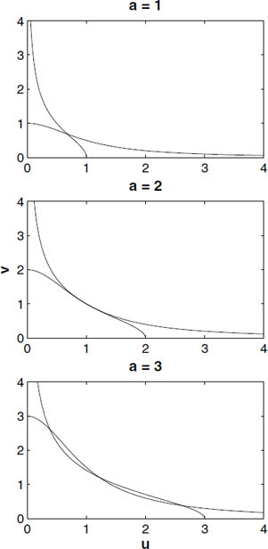
Figure 4.8 Plots of the nullclines for the model [4.5] in the (u, v) plane for values of a below, above, and exactly at the bifurcation between one and three equilibria for the model.

Exercise 4.3. For what parameter combinations (a, b) do the two nullclines have exactly the same slope at the symmetric equilibrium?

Figure 4.9 Bifurcation diagram of the (b, a) plane for the model [4.5]. For values of (b, a) below the bifurcation curve, there is a single equilibrium point, while for values of (b, a) above the bifurcation curve, there are three equilibrium points.

The conclusion of this exercise is that the bifurcation of the symmetric equilibrium occurs where

a = b(b − 1)^−(1+b)/b.

Figure 4.9 shows the graph of this function. Note that, when b = 2, the bifurcation occurs at a = 2. For values of (a, b) below the bifurcation curve, there is a single equilibrium point, while for values of (a, b) above the bifurcation curve, there are three equilibrium points.

Figures 4.10 and 4.11 show phase portraits in these two cases. In Figure 4.10 the symmetric equilibrium is stable, and all solutions tend toward it. In Figure 4.11, the symmetric equilibrium has become unstable but the two other equilibria are both stable. Some initial conditions produce trajectories that approach one stable state while other initial conditions produce trajectories that approach the second stable state. The bifurcation that occurs in the model is called a pitchfork bifurcation because one equilibrium splits into three as a parameter is varied. Pitchfork bifurcations are typically found at symmetric equilibria in systems that have a symmetry. Figure 4.11 also shows the nullclines of the system. The three equilibrium points lie at the intersections of the nullclines. These figures illustrate the visualization of phase portraits for systems of two differential equations. We see the paths taken by points (u, v) as they move along solutions to the system of equations. The techniques that we have applied here,

Figure 4.10 Phase portrait of the (u, v) plane for the model [4.5] with (b, a) = (3, 1). There is a single equilibrium point, which is stable and lies on the line u = v.

Figure 4.11 Phase portrait of the (u, v) plane for the model [4.5] with (e, a) = (3, 2). There are three equilibrium points, located at the intersections of the nullclines (the curves that reach the boundary of the bounding box).

• nondimensionalizing the model to reduce the number of parameters,

• plotting the nullclines to locate equilibria, and

• determining the local stability of the equilibria as a function of parameter values,

are often all it takes to determine the important properties of a model’s solutions.

As with the repressilator, the model [4.5] gives clues about how to choose repressors in this regulatory network that will make a good toggle switch. In particular, increasing protein synthesis rates makes the two stable states of the system move farther apart in the phase plane. The enhanced distance between the repressor concentrations makes it both easier to distinguish the two stable states and harder for perturbations to push the switch from one state to another. Large distance between the stable states makes it hard for “noise” to cause the system to switch spontaneously between them; larger inputs are needed to switch the system when one desires to do so. It is not evident on the phase plane plots, but increasing a also makes the switching between the states faster. Increasing the cooperativity parameter b makes the bifurcation value of the protein synthesis rate a decrease. We conclude that large a and b both work to make the switch more robust but perhaps harder to purposefully switch between states.

Exercise 4.4. Explore the behavior of the solutions to the system [4.5] when the parameters α_u ≠ α_v and β ≠ γ. Can you find significantly different types of dynamical behavior than in the cases where each pair of parameters is equal?

4.4 Systems Biology

“Systems biology” is a new term, created in the past few years to describe an area of research whose boundaries remain fuzzy. Although organs, organisms, and ecosystems are all systems—in the conventional sense that we can regard them as composed of interacting elements—systems biology tends to focus on processes at the cellular level. The new journal Systems Biology has the following introduction:

Systems biology involves modelling and simulating the complex dynamic interactions between genes, transcripts, proteins, metabolites and cells using integrated systems-based approaches. Encompassing proteomics, transcriptomics, metabolomics and functional genomics, systems biology uses computational and mathematical models to analyze and simulate networks, pathways and the spatial and temporal relationships that give rise to cause and effect in living systems. Such work is of great importance to a better understanding of disease mechanisms, pharmaceutical drug discovery and drug target validation.

The “omics” listed above refer to methods for collecting and analyzing large amounts of data about the molecular biology of cells. Whole genome sequences of many organisms are one striking example of such data. The humane genome has billions of nucleotides and thousands of genes. Computational tools are needed to manage these data, and even tasks like searching for similar sequences in different genomes require efficient algorithms. Systems biology seeks to discover the organization of these complex systems. Cells have intricate internal structure, with organelles like ribosomes and mitochondria and smaller molecular complexes like DNA polymerase that play an essential role in how cells function. Structural information is not enough, however, to understand how cells work. Life is inherently a dynamic process. There are varied approaches that systems biology is taking to model and simulate these dynamics. Systems biology research has been accelerating rapidly, but this is an area of research that is in its infancy and fundamentally new ideas may be needed to close the enormous gap between goals that have been articulated and present accomplishments.

The models of gene regulation in this chapter are simple examples of systems biology models. One simplified view of the cell is to regard it as a soup of reacting chemicals. This leads us to model the cell as sets of chemical reactions as we have done with our simple gene regulation circuits. Conceptually, we can try to “scale up” from systems with two or three genes and their represssors to whole cells with thousands of genes, molecules, and molecular complexes that function as distinct entities in cellular dynamics. Practically, there are enormous challenges in constructing models that faithfully reproduce the dynamical processes we observe in cells. We give a brief overview of some of these challenges for systems biology research in this section, from our perspective as dynamicists.

Much of current systems biology research is directed at discovering “networks” and “pathways.” Viewing the cell as a large system of interactions among components like chemical reactions, its dynamics is modeled as a large set of ordinary differential equations. There is a network structure to these equations that comes from mass balance. Each interaction transforms a small group of cellular components into another small group. We can represent the possible transforms as a directed graph in which there is a vertex for each component and an arrow from component A to component B if there is an interaction that directly transforms A to B. We can seldom see directly the interactions that take place in the cell, but there are two classes of techniques that enable us to infer some of the network structure. First, we can detect correlations of the concentrations of different entities with “high-throughput” measurements. Example techniques include microarrays that measure large numbers of distinct mRNA molecules and the simultaneous measurements of the concentration of large numbers of proteins with mass spectrometry. Second, genetic modifications of an organism enable us to decrease or enhance expression of individual genes and to modify proteins in specific ways. The effects of these genetic modifications yield insight into the pathways and processes that involve specific genes and proteins.

Exercise 4.5. Draw a graph that represents the interactions between components of the repressilator network.

Construction of networks for gene regulation and cell signaling is one prominent activity for systems biology. Networks with hundreds to thousands of nodes have been constructed to represent such processes as the cell cycle (Kohn 1999) and the initiation of cancer (http://www.gnsbiotech.com/biology.php). For the purposes of creating new drugs, such networks help to identify specific targets in pathways that malfunction during a disease. Can we do more? What can we infer about how a system works from the structure of its network? We can augment the information in the network by classifying different types of entities and their interactions and using labels to identify these on a graph. Feedback in a system can be identified with loops in the graph, and we may be able to determine from the labels whether feedback is positive or negative; i.e., whether the interactions serve to enhance or suppress the production of components within the loop. However, as we have seen with the simple switch and repressilator networks, a single network can support qualitatively different dynamics that depend on quantitative parameters such as reaction rates. Thus, we would like to develop dynamic models for cellular processes that are consistent with the network graphs.

Differential equation models for a reaction network require rate laws that describe how fast each reaction proceeds. In many situations we cannot derive the rate laws from first principles, so we must either measure them experimentally or choose a rate law based on the limited information that we do have. Isolating the components of reactions in large network models and measuring their kinetics is simply not feasible. As in the two models considered earlier in this chapter, the Michaelis-Menten rate law for enzyme kinetics derived in Chapter 1 and mass action kinetics are frequently used in systems biology models. The functional forms chosen for rate laws usually have parameters that still must be given values before simulations of the model are possible. With neural models for the electrical excitability of a neuron, the voltage clamp technique is used to estimate many of the model parameters, but better experimental techniques are needed for estimating parameters in the rate laws of individual cellular interactions. Thus, estimating model parameters is one of the challenges we confront when constructing dynamic models of cellular networks.

Transformation of networks and rate laws into differential equations models is a straightforward but tedious and error-prone process when done “by hand.” Moreover, comparison and sharing of models among researchers is much easier when standards are formulated for the computer description of models. Accordingly, substantial effort has been invested in the development of specialized languages for defining systems biology models. One example is SBML, the Systems Biology Markup Language, that is designed to provide a “tool-neutral” computer-readable format for representing models of biochemical reaction networks (http://sbml.org/index.psp).

Exercise 4.6. Describe the types of computations performed by three different systems biology software tools. You can find links to many tools on the homepage of the SBML website.

Once a model is constructed we face the question as to whether the simulations are consistent with experimental observations. Since even a modest-size model is likely to have dozens of unmeasured parameters, we can hardly expect that the initial choices that have been made for all of these will combine to yield simulations that do match data. What do we do to “tune” the model to improve the fit between simulations and data? The simplest thing that can be done is to compute simulations for large numbers of different parameters, observing the effects of parameter changes. We can view the computer simulations as a new set of experiments and use the speed of the computer to do lots of them. As the number of parameters increases, a brute force “sweep” through the parameter space becomes impossible. For example, simulating a system with each of ten different values of k parameters that we vary independently requires 10^k simulations altogether. Thus, brute force strategies to identify parameters can only take us so far.

When simulations have been carried out for differential equation models arising in many different research areas, similar patterns of dynamical behavior have been observed. For example, the way in which periodic behavior in the repressilator arises while varying parameters is similar to the way in which it arises in the Morris-Lecar model for action potentials. Dynamical systems theory provides a mathematical framework for explaining these observations that there are “universal” qualitative properties that are found in simulation of differential equations models. We use this theory to bolster our intuition about how properties of the simulations depend upon model parameters. Tyson, Chen, and Novak (2001) review model studies of the cell cycle in yeast, illustrating how dynamical systems theory helps interpret the results of simulations of these models.

Mathematics can also help estimate parameters in a model in another way. If we are interested in the quantitative fit of a model to data, then we can formulate parameter estimation as an optimization problem. We define an objective function that will be used to measure the difference between a simulation and data. A common choice of objective function is least squares. If x₁, . . . , x_n are observations and y₁, . . . , y_n are the corresponding values obtained from simulation, then the least squares objective function is Σ(y_i − x_i)². It is often useful to introduce weights w_i > 0 and consider the weighted least squares objective function Σw_i(y_i − x_i)². The value of this objective function is non-negative and the simulation fits the data perfectly if and only if the value of the objective function is zero. The value of any objective function f will depend upon the parameters of a model. The optimization problem is to find the parameters that give the minimum value of the objective function. There are several well-developed computational strategies for solving this optimization problem, but it would take us far afield to pursue them here. Some of the computational tools that have been developed for systems biology (http://www.gepasi.org/,http://www.copasi.org) attempt to solve parameter estimation problems using some basic optimization algorithms. The methods have been tested successfully on systems of a few chemical reactions, but we still do not know whether they will make significant improvements in estimating parameters of large models. Some of the difficulties encountered in application of optimization methods to estimating parameter of network models are addressed by Brown and Sethna (2003).

4.4.1 Complex versus Simple Models

Finding basic “laws” for systems biology is a compelling challenge. There is still much speculation about what those principles might be and how to find them. There is wide agreement that computational models are needed to address this challenge, but there is divergence of opinion as to the complexity of the models we should focus upon.

Taking advantage of experimental work aimed at identifying interaction networks in cells, systems biologists typically formulate and study models with many state variables that embrace the complexity of the system being modeled, rather than trying to identify and model a few “key” variables. Nobody denies the necessity of complex models for applied purposes, where any and all biological details should be incorporated that improve a model’s ability to make reliable predictions, though as we discuss in Chapter 9, putting in too much biological detail can sometimes be bad for forecasting accuracy. For example, in a human cancer cell model developed to help design and optimize patient-specific chemotherapy (Christopher et al. 2004), the diagram for the cell apoptosis module includes about forty interlinked state variables and links to two other submodels of undescribed complexity (“cell cycle module” and “p53 module”).

But for basic research, there is a long-standing and frequently heated debate over the value of simple “general” models versus complex “realistic” models as tools. On one side Lander (2004, p. 712) dismisses both simple models and the quest for generality:

. . . starting from its heyday in the 1960s, [mathematical biology] provided some interesting insights, but also succeeded in elevating the term “modeling” to near-pejorative status among many biologists. For the most part mathematical biologists sought to fit biological data to relatively simple models, with the hope that fundamental laws might be recognized . . . . This strategy works well in physics and chemistry, but in biology it is stymied by two problems. First, biological data are usually incomplete and extremely imprecise. As new measurements are made, today’s models rapidly join tomorrow’s scrap heaps. Second, because biological phenomena are generated by large, complex networks of elements there is little reason to expect to discern fundamental laws in them. To do so would be like expecting to discern the fundamental laws of electromagnetism in the output of a personal computer.

In order to “elevate investigations in computation biology to a level where ordinary biologists take serious notice”, the “essential elements” include “network topologies anchored in experimental data” and “fine-grained explorations of large parameter spaces” (Lander 2004, p. 714).

The alternative view is that there are basic “pathways,” “motifs,” and “modules” in cellular processes that are combined as building blocks in the assembly of larger systems, and that there are definite principles in the way in which they are combined. In contrast to Lander, we would say that biological phenomena are generated by evolution, which uses large complex networks for some tasks; this distinction is crucial for the existence of fundamental laws and the levels at which they might be observed. Evolution has the capacity to dramatically alter the shape and behavior of organisms in a few generations, but there are striking similarities in the molecular biology of all organisms, and cross-species comparisons show striking similarities in individual genes. Natural selection has apparently preserved—or repeatedly discovered—successful solutions to the basic tasks that cells face. Biological systems are therefore very special networks which may have general organizational principles.

We build complex machines as assemblies of subsystems that interact in ways that do not depend upon much of the internal structure of the subsystems. We also create new devices using preexisting components—consider the varied uses of teflon, LCDs, and the capacitor. Many biologists (e.g., Alon 2003) have argued that designs produced by evolution exhibit the same properties—modularity and recurring design elements—because good design is good design, whether produced by human intelligence or the trial-and-error of mutation and natural selection. Alon (2003) notes in particular that certain network elements that perform particular tasks, such as buffering the network against input fluctuations, occur repeatedly in many different organisms and appear to have evolved independently numerous times, presumably because they perform the task well. The existence of recurring subsystems with well-defined functions opens the possibility of decomposing biological networks in a hierarchical fashion: using small models to explore the interactions within each kind of subsystem, and different small models to explore the higher-level interactions among subsystems that perform different functions. How well this strategy works depends on the extent to which whole-system behavior is independent of within-subsystem details, which still remains to be seen.

Proponents of simpler models often question the utility of large computer simulations, viewing them as a different type of complex system that is far less interesting than the systems they model. In the context of ecological models, mathematical biologist Robert May (1974, p. 10) expressed the opinion that many “massive computer studies could benefit most from the installation of an on-line incinerator” and that this approach “does not seem conducive to yielding general ecological principles.” In principle one can do “fine-grained explorations of large parameter spaces” to understand the behavior of a computational model, as Lander (2004) recommends; in practice it is impossible to do the 10⁵⁰ simulation runs required to try out all combinations of 10 possible values for each of 50 parameters. Similarly Gavrilets (2003) argued that the theory of speciation has failed to advance because of over-reliance on complex simulation models:

The most general feature of simulation models is that their results are very specific. Interpretation of numerical simulations, the interpolation of their results for other parameter values, and making generalizations based on simulations are notoriously difficult . . . simulation results are usually impossible to reproduce because many technical details are not described in original publications.

According to Gavrilets (2003) the crucial step for making progress is “the development of simple and general dynamical models that can be studied not only numerically but analytically as well.” Ginzburg and Jensen (2004) compare complex models with large parameter spaces to the Ptolemaic astronomy based on multilayered epicycles: adaptable enough to fit any data, and therefore meaningless.

Of course the quotes above were carefully selected to showcase extreme positions. Discussions aiming for the center are also available—indeed, the quotes above from May (1974) were pulled from a balanced discussion of the roles of simple versus complex models, and we also recommend Hess (1996), Peck (2004), and the papers by Hall (1988) and Caswell (1988) that deliberately stand at opposite ends of the field and take aim at each other. The relative roles that simple and complex dynamic models will play in systems biology are uncertain, but it seems that both will be used increasingly as we accumulate more information about the networks and pathways of intracellular interactions.

4.5 Summary

This chapter has explored the dynamics of differential equation models for two synthetic gene regulation networks. The models were chosen to illustrate how simulation is used to study nonlinear differential equations. The focus is upon long-time, asymptotic properties of the solutions. We distinguish solutions that tend to an equilibrium, or steady state, from solutions that tend to periodic orbits. In the next chapter, we give an introduction to the mathematics of dynamical systems theory as a conceptual framework for the study of such questions. The theory emphasizes qualitative properties of solutions to differential equations like the distinction between solutions that tend to equilibria and those that tend to periodic orbits. The results of simulations are fitted into a geometric picture that shows the asymptotic properties of all solutions.

The application of dynamical systems methods to gene regulatory networks is a subject that is still in its infancy. To date, systems biology has been more effective in developing experimental methods for determining networks of interactions among genes, proteins, and other cellular components than in developing differential equation models for these complex systems. Simulation is essentially the only general method for determining solutions of differential equations. Estimating parameters in large models that lead to good fits with data is an outstanding challenge for systems biology. We do not know whether there are general principles underlying the internal organization of cells that will help us to build better models of intracellular systems. The mathematics of dynamical systems theory and optimization theory do help us in investigations of large models of these systems.

4.6 References

Alon, U. 2003. Biological networks: the tinkerer as an engineer. Science 301: 1866–1867.

Atkinson, M., M. Savageau, J. Myers, and A. Ninfa. 2003. Development of genetic circuitry exhibiting toggle switch or oscillatory behavior in Escherichia coli. Cell 113: 597–607.

Brown, K., and J. Sethna. 2003. Statistical mechanics approaches to models with many poorly known parameters. Physical Review E 68: 021904.

Caswell, H. 1988. Theory and models in ecology: A different perspective. Ecological Modelling 43: 33–44.

Christopher, R., A. Dhiman, J. Fox, R. Gendelman, T. Haberitcher, D. Kagle, G. Spizz, I. G. Khalil, and C. Hill. 2004. Data-driven computer simulation of human cancer cell. Annals of the NY Academy of Science 1020: 132–153.

Elowitz, M., and S. Leibler. 2000. A synthetic oscillatory network of transcriptional regulators. Nature 403: 335–338.

Ferber, D. 2004. Microbes made to order. Science 303: 158–161.

Gardner, T., C. Cantor, and J. Collins. 2000. Construction of a genetic toggle switch in Escherichia coli. Nature 403: 339–342.

Gavrilets, S. 2003. Models of speciation: What have we learned in 40 years? Evolution 57: 2197–2215.

Ginzburg, L. R., and C.X.J. Jensen. 2004. Rules of thumb for judging ecological theories. Trends in Ecology and Evolution 19: 121–126.

Hall, C.A.S. 1988. An assessment of several of the historically most influential theoretical models in ecology and of the data provided in their support. Ecological Modelling 43: 5–31.

Hasty, J., D. McMillen, and J. Collins. 2002. Engineered gene circuits. Nature 402: 224–230.

Hess, G. R. 1996. To analyze, or to stimulate, is that the question? American Entomologist 42: 14–16.

Kohn, K. 1999. Molecular interaction map of the mammalian cell cycle control and DNA repair system. Molecular Biology of the Cell 10: 2703–2734.

Lander, A. D. 2004. A calculus of purpose. PLoS Biology 2: 712–714.

May, R. M. 1974. Stability and Complexity in Model Ecosystems, 2nd edition. Princeton University Press, Princeton, NJ.

Peck, S. L. 2004. Simulation as experiment: A philosophical reassessment for biological modeling. Trends in Ecology and Evolution 19: 530–534.

Tyson, J. J., K. Chen, and B. Novak. 2001. Network dynamics and cell physiology. Nature Reviews: Molecular Cell Biology 2: 908–916.

¹Interest in pathways is intense: the Science Magazine Signal Transduction Knowledge Environment provides an online interface (http://stke.sciencemag.org/cm/) to databases of information on the components of cellular signaling pathways and their relations to one another.

²Units of time and concentration in the model have been “scaled” to make these equations “nondimensional.” This means that the variables m_i, p_i, and time have been multiplied by fixed scalars to reduce the number of parameters that would otherwise be present in the equations. One of the reductions is to make the time variable correspond to the decay rate of the mRNA so that the coefficient of m_i in the equation for is –1: when time is replaced by τ = at in the equation

the result is

³We will discuss linearization and the mathematical theory of linear systems of differential equations in Chapter 5.

⁴For those of you who have studied differential equations, the proof is short: the divergence of the system [4.5] is negative, so areas in the phase plane shrink under the flow. However, the region bounded within a periodic solution would be invariant and maintain constant area under the flow.