This chapter discusses the key factors used for understanding disk behavior and presents an overview of the analysis tools available.
The following terms are related to disk analysis; the list also summarizes topics covered in this section.
Environment. The first step in disk analysis is to know what the disks are—single disks or a storage array—and what their expected workload is: random, sequential, or otherwise.
Utilization. The percent busy value from
iostat -xserves as a utilization value for disk devices. The calculation behind it is based on the time a device spends active. It is a useful starting point for understanding disk usage.Saturation. The average wait queue length from
iostat -xis a measure of disk saturation.Throughput. The kilobytes/sec values from
iostat -xcan also indicate disk activity, and for storage arrays they may be the only meaningful metric that Solaris provides.I/O rate. The number of disk transactions per second can be seen by means of
iostator DTrace. The number is interesting because each operation incurs a certain overhead. This term is also known as IOPS (I/O operations per second).I/O sizes. You can calculate the size of disk transactions from
iostat -xby using the (kr/s + kw/s) / (r/s + w/s) ratio, which gives average event size; or you can measure the size directly with DTrace. Throughput is usually improved when larger events are used.Service times. The average wait queue and active service times can be printed from
iostat -x. Longer service times are likely to degrade performance.History.
sarcan be activated to archive historical disk activity statistics. Long-term patterns can be identified from this data, which also provides a reference for what statistics are “normal” for your disks.Seek sizes. DTrace can measure the size of each disk head seek and present this data in a meaningful report.
I/O time. Measuring the time a disk spends servicing an I/O event is valuable because it takes into account various costs of performing an I/O operation: seek time, rotation time, and the time to transfer data. DTrace can fetch event time data.
Table 4.1 summarizes and cross-references tools used in this section.
Table 4.1. Tools for Disk Analysis
Tool | Uses | Description | Reference |
|---|---|---|---|
| Kstat | For extended disk device statistics | 4.6 |
| Kstat, sadc | For disk device statistics and history data archiving | 4.13 |
| DTrace | Simple script for events by device and file name | 4.15.3 |
| DTrace | Simple script to aggregate disk event size | 4.15.4 |
| DTrace | Simple script to measure disk event seek size | 4.15.5 |
| DTrace | Simple script to aggregate size by file name | 4.15.6 |
| DTrace | For a disk statistics by-process summary | 4.17.1 |
| DTrace | For a trace of disk events, including process ID, times, block addresses, sizes, etc. | 4.17.2 |
We frequently use the terms random and sequential while discussing disk behavior. Random activity means the disk accesses blocks from random locations on disk, usually incurring a time penalty while the disk heads seek and the disk itself rotates. Sequential activity means the disk accesses blocks one after the other, that is, sequentially.
The following demonstrations compare random to sequential disk activity and illustrate why recognizing this behavior is important.
While a dd command runs to request heavy sequential disk activity, we examine the output of iostat to see the effect. (The options and output of iostat are covered in detail in subsequent sections.)
# dd if=/dev/rdsk/c0d0s0 of=/dev/null bs=64k
$ iostat -xnz 5
                    extended device statistics
    r/s    w/s   kr/s   kw/s wait actv wsvc_t asvc_t  %w  %b device
    1.1    0.7   16.2   18.8  0.3  0.0  144.4    2.7   0   0 c0d0
    0.0    0.0    0.0    0.0  0.0  0.0    0.0    0.2   0   0 jupiter:vold(pid564)
                    extended device statistics
    r/s    w/s   kr/s   kw/s wait actv wsvc_t asvc_t  %w  %b  device
  819.6    0.0 52453.3    0.0  0.0  1.0    0.0    1.2   1  97  c0d0
                    extended device statistics
    r/s    w/s   kr/s   kw/s wait actv wsvc_t asvc_t  %w  %b device
  820.9    0.2 52535.2    1.6  0.0  1.0    0.0    1.2   1  97 c0d0
                    extended device statistics
    r/s    w/s   kr/s   kw/s wait actv wsvc_t asvc_t  %w  %b device
  827.8    0.0 52981.2    0.0  0.0  1.0    0.0    1.2   1  97 c0d0
...
The disk was 97% busy, for which it delivered over 50 Mbytes/sec.
Now for random activity, on the same system and the same disk. This time we use the filebench tool to generate a consistent and configurable workload.
filebench> load randomread
filebench> set $nthreads=64
filebench> run 600
 1089: 0.095: Random Read Version 1.8 05/02/17 IO personality successfully loaded
 1089: 0.096: Creating/pre-allocating files
 1089: 0.279: Waiting for preallocation threads to complete...
 1089: 0.279: Re-using file /filebench/bigfile0
 1089: 0.385: Starting 1 rand-read instances
 1090: 1.389: Starting 64 rand-thread threads
 1089: 4.399: Running for 600 seconds...

$ iostat -xnz 5
                    extended device statistics
    r/s    w/s   kr/s   kw/s wait actv wsvc_t asvc_t  %w  %b device
    1.0    0.7    8.6   18.8  0.3  0.0  154.2    2.8   0   0 c0d0
    0.0    0.0    0.0    0.0  0.0  0.0    0.0    0.2   0   0 jupiter:vold(pid564)
                    extended device statistics
    r/s    w/s   kr/s   kw/s wait actv wsvc_t asvc_t  %w  %b  device
  291.6    0.2 1166.5    1.6  0.0  1.0    0.0    3.3   0  97  c0d0
                    extended device statistics
    r/s    w/s   kr/s   kw/s wait actv wsvc_t asvc_t  %w  %b device
  290.0    0.0 1160.1    0.0  0.0  1.0    0.0    3.3   0  97 c0d0
...
This disk is also 97% busy, but this time it delivers around 1.2 Mbytes/sec. The random disk activity was over 40 times slower in terms of throughput. This is quite a significant difference.
Had we only been looking at disk throughput, then 1.2 Mbytes/sec may have been of no concern for a disk that can pull 50 Mbytes/sec; in reality, however, our 1.2 Mbytes/sec workload almost saturated the disk with activity. In this case, the percent busy (%b) measurement was far more useful, but for other cases (storage arrays), we may find that throughput has more meaning.
Larger environments often use storage arrays: These are usually hardware RAID along with an enormous frontend cache (256 Mbytes to 256+ Gbytes). Rather than the millisecond crawl of traditional disks, storage arrays are fast—often performing like an enormous hunk of memory. Reads and writes are served from the cache as much as possible, with the actual disks updated asynchronously.
If we are writing data to a storage array, Solaris considers it completed when the sd or ssd driver receives the completion interrupt. Storage arrays like to use writeback caching, which means the completion interrupt is sent as soon as the cache receives the data. The service time that iostat reports will be tiny because we did not measure a physical disk event. The data remains in the cache until the storage array flushes it to disk at some later time, based on algorithms such as Least Recently Used. Solaris can’t see any of this. Solaris metrics such as utilization may have little meaning; the best metric we do have is throughput—kilobytes written per second—which we can use to estimate activity.
In some situations the cache can switch to writethrough mode, such as in the event of a hardware failure (for example, the batteries die). Suddenly the statistics in Solaris change because writes now suffer a delay as the storage array waits for them to write to disk, before an I/O completion is sent. Service times increase, and utilization values such as percent busy may become more meaningful.
If we are reading data from a storage array, then at times delays occur as the data is read from disk. However, the storage array tries its best to serve reads from (its very large) cache, especially effective if prefetch is enabled and the workload is sequential. This means that usually Solaris doesn’t observe the disk delay, and again the service times are small and the percent utilizations have little meaning.
To actually understand storage array utilization, you must fetch statistics from the storage array controller itself. Of interest are cache hit ratios and array controller CPU utilization. The storage array may experience degraded performance as it performs other tasks, such as verification, volume creation, and volume reconstruction. How the storage array has been configured and its underlying volumes and other settings are also of great significance.
The one Solaris metric we can trust for storage arrays is throughput, the data read and written to it. That can be used as an indicator for activity. What happens beyond the cache and to the actual disks we do not know, although changes in average service times may give us a clue that some events are synchronous.
Sector zoning, also known as Multiple Zone Recording (MZR), is a disk layout strategy for optimal performance. A track on the outside edge of a disk can contain more sectors than one on the inside because a track on the outside edge has a greater length. Since the disk can read more sectors per rotation from the outside edge than the inside, data stored near the outside edge is faster. Manufacturers often break disks into zones of fixed sector per-track ratios, with the number of zones and ratios chosen for both performance and data density.
Data throughput on the outside edge may also be faster because many disk heads rest at the outside edge, resulting in reduced seek times for data blocks nearby.
A simple way to demonstrate the effect of sector zoning is to perform a sequential read across the entire disk. The following example shows the throughput at the start of the test (outside edge) and at the end of the test (inside edge).
# dd if=/dev/rdsk/c0t0d0s2 of=/dev/null bs=128k
$ iostat -xnz 10
...
                    extended device statistics
    r/s    w/s   kr/s   kw/s wait actv wsvc_t asvc_t  %w  %b device
  104.0    0.0 13311.0    0.0  0.0  1.0    0.0    9.5   0  99 c0t0d0
...
                    extended device statistics
    r/s    w/s   kr/s   kw/s wait actv wsvc_t asvc_t  %w  %b device
   71.1    0.0 9100.4    0.0  0.0  1.0    0.0   13.9   0  99 c0t0d0
Near the outside edge the speed was around 13 Mbytes/sec, while at the inside edge this has dropped to 9 Mbytes/sec. A common procedure that takes advantage of this behavior is to slice disks so that the most commonly accessed data is positioned near the outside edge.
An important characteristic when storage devices are configured is the maximum size of an I/O transaction. For sequential access, larger I/O sizes are better; for random access, I/O sizes should to be picked to match the workload. Your first step when configuring I/O sizes is to know your workload: DTrace is especially good at measuring this (see Section 4.15).
A maximum I/O transaction size can be set at a number of places:
maxphys. Disk driver maximum I/O size. By default this is 128 Kbytes on SPARC systems and 56 Kbytes on x86 systems. Some devices override this value if they can.
maxcontig. UFS maximum I/O size. Defaults to equal maxphys, it can be set during
newfs(1M)and changed withtunefs(1M). UFS uses this value for read-ahead.stripe width. Maximum I/O size for a logical volume (hardware RAID or software VM) configured by setting a stripe size (per-disk maximum I/O size) and choosing a number of disks. stripe width = stripe size × number of disks.
interlace. SVM stripe size.
Ideally, stripe width is an integer divisor of the average I/O transaction size; otherwise, there is a remainder. Remainders can reduce performance for a few reasons, including inefficient filling of cache blocks; and in the case of RAID5, remainders can compromise write performance by incurring the penalty of a read-modify-write or reconstruct-write operation.
The following is a quick demonstration to show maxphys capping I/O size on Solaris 10 x86.
# dd if=/dev/dsk/c0d0s0 of=/dev/null bs=1024k

$ iostat -xnz 5
                    extended device statistics
    r/s    w/s   kr/s   kw/s wait actv wsvc_t asvc_t  %w  %b device
    2.4    0.6   55.9   17.8  0.2  0.0   78.9    1.8   0   0 c0d0
    0.0    0.0    0.0    0.0  0.0  0.0    0.0    0.2   0   0 jupiter:vold(pid564)
                    extended device statistics
    r/s    w/s   kr/s   kw/s wait actv wsvc_t asvc_t  %w  %b device
  943.3    0.0 52822.6    0.0  0.0  1.3    0.0    1.4   3 100 c0d0
                    extended device statistics
    r/s    w/s   kr/s   kw/s wait actv wsvc_t asvc_t  %w  %b device
  959.2    0.0 53716.1    0.0  0.0  1.3    0.0    1.4   3 100 c0d0
                    extended device statistics
    r/s    w/s   kr/s   kw/s wait actv wsvc_t asvc_t  %w  %b device
  949.8    0.0 53186.3    0.0  0.0  1.2    0.0    1.3   3  96 c0d0
...
Although we requested 1024 Kbytes per transaction, the disk device delivered 56 Kbytes (52822 ÷ 943), which is the value of maxphys.
The dd command can be invoked with different I/O sizes while the raw (rdsk) device is used so that the optimal size for sequential disk access can be discovered.
The iostat utility is the official place to get information about disk I/O performance, and it is a classic kstat(3kstat) consumer along with vmstat and mpstat. iostat can be run in a variety of ways.
In the following style, iostat provides single-line summaries for active devices.
$ iostat -xnz 5
                    extended device statistics
    r/s    w/s   kr/s   kw/s wait actv wsvc_t asvc_t  %w  %b  device
    0.2    0.2    1.1    1.4  0.0  0.0    6.6    6.9   0   0  c0t0d0
    0.0    0.0    0.0    0.0  0.0  0.0    0.0    7.7   0   0  c0t2d0
    0.0    0.0    0.0    0.0  0.0  0.0    0.0    3.0   0   0  mars:vold(pid512)
                    extended device statistics
    r/s    w/s   kr/s   kw/s wait actv wsvc_t asvc_t  %w  %b  device
  277.1    0.0 2216.4    0.0  0.0  0.6    0.0    2.1   0  58  c0t0d0
                    extended device statistics
    r/s    w/s   kr/s   kw/s wait actv wsvc_t asvc_t  %w  %b  device
   79.8    0.0  910.0    0.0  0.4  1.9    5.1   23.6  41  98  c0t0d0
                    extended device statistics
    r/s    w/s   kr/s   kw/s wait actv wsvc_t asvc_t  %w  %b  device
   87.0    0.0  738.5    0.0  0.8  2.0    9.4   22.4  65  99  c0t0d0
                    extended device statistics
    r/s    w/s   kr/s   kw/s wait actv wsvc_t asvc_t  %w  %b  device
   92.2    0.6  780.4    2.2  2.1  1.9   22.8   21.0  87  98  c0t0d0
                    extended device statistics
    r/s    w/s   kr/s   kw/s wait actv wsvc_t asvc_t  %w  %b  device
  101.4    0.0  826.6    0.0  0.8  1.9    8.0   19.0  46  99  c0t0d0
...
The first output is the summary since boot, followed by samples every five seconds. Some columns have been highlighted in this example. On the right is %b; this is percent busy and tells us disk utilization, [1] which we explain in the next section. In the middle is wait, the average wait queue length; it is a measure of disk saturation. On the left are kr/s and kw/s, kilobytes read and written per second, which tells us the current disk throughput.
In the iostat example, the first five-second sample shows a percent busy of 58%—fairly moderate utilization. For the following samples, we can see the average wait queue length climb to a value of 2.1, indicating that this disk was becoming saturated with requests.
The throughput in the example began at over 2 Mbytes/sec and fell to less than 1 Mbytes/sec. Throughput can indicate disk activity.
iostat provides other statistics that we discuss later. These utilization, saturation, and throughput metrics are a useful starting point for understanding disk behavior.
When considering disk utilization, keep in mind the following points:
Any level of disk utilization may degrade application performance because accessing disks is a slow activity—often measured in milliseconds.
Sometimes heavy disk utilization is the price of doing business; this is especially the case for database servers.
Whether a level of disk utilization actually affects an application greatly depends on how the application uses the disks and how the disk devices respond to requests. In particular, notice the following:
– An application may be using the disks synchronously and suffering from each delay as it occurs, or an application may be multithreaded or use asynchronous I/O to avoid stalling on each disk event.
– Many OS and disk mechanisms provide writeback caching so that although the disk may be busy, the application does not need to wait for writes to complete.
Utilization values are averages over time, and it is especially important to bear this in mind for disks. Often, applications and the OS access the disks in bursts: for example, when reading an entire file, when executing a new command, or when flushing writes. This can cause short bursts of heavy utilization, which may be difficult to identify if averaged over longer intervals.
Utilization alone doesn’t convey the type of disk activity—in particular, whether the activity was random or sequential.
An application accessing a disk sequentially may find that a heavily utilized disk often seeks heads away, causing what would have been sequential access to behave in a random manner.
Storage arrays may report 100% utilization when in fact they are able to accept more transactions. 100% utilization here means that Solaris believes the storage device is fully active during that interval, not that it has no further capacity to accept transactions. Solaris doesn’t see what really happens on storage array disks.
Disk activity is complex! It involves mechanical disk properties, buses, and caching and depends on the way applications use I/O. Condensing this information to a single utilization value verges on oversimplification. The utilization value is useful as a starting point, but it’s not absolute.
In summary, for simple disks and applications, utilization values are a meaningful measurement so we can understand disk behavior in a consistent way. However, as applications become more complex, the percent utilization requires careful consideration. This is also the case with complex disk devices, especially storage arrays, for which percent utilization may have little value.
While we may debate the accuracy of percent utilization, it still often serves its purpose as being a “useful starting point,” which is followed by other metrics when deeper analysis is desired (especially those from DTrace).
A sustained level of disk saturation usually means a performance problem. A disk at saturation is constantly busy, and new transactions are unable to preempt the currently active disk operation in the same way a thread can preempt the CPU. This means that new transactions suffer an unavoidable delay as they queue, waiting their turn.
Throughput is interesting as an indicator of activity. It is usually measured in kilobytes or megabytes per second. Sometimes it is of value when we discover that too much or too little throughput is happening on the disks for the expected application workload.
Often with storage arrays, throughput is the only statistic available from iostat that is accurate. Knowing utilization and saturation of the storage array’s individual disks is beyond what Solaris normally can see. To delve deeper into storage array activity, we must fetch statistics from the storage array controller.
The iostat command can print a variety of different outputs, depending on which command-line options were used. Many of the standard options are listed below.[2]
-c. Print the standard system time percentages:us,sy,wt,id.-d. Print classic fields:kps,tps,serv.-D. “New” style output, print disk utilization with a decimal place.-e. Print device error statistics.-E. Print extended error statistics. Useful for quickly listing disk details.-I. Print raw interval counts, rather than per second.-ln. Limit number of disks printed ton. Useful when also specifying a disk.-M. Print throughput in Mbytes/sec rather than Kbytes/sec.-n. Use logical disk names rather than instance names.-p. Print per partition statistics as well as per device.-P. Print partition statics only.-t. Print terminal I/O statistics.-x. Extended disk statistics. This prints a line per device and provides the breakdown that includesr/s,w/s,kr/s,kw/s,wait,actv,svc_t,%w, and%b.
The default options of iostat are -cdt, which prints a summary of up to four disks on one line along with CPU and terminal I/O details. This is rarely used.[3]
Several new formatting flags crept in around Solaris 8:
-C. Report disk statistics by controller.-m. For mounted partitions, print the mount point (useful with-por-P).-r. Display data in comma-separated format.-s. Suppress state change messages.-T d | u. Print timestamps in date (d) or UNIX time (u) format.-z. Don’t print lines that contain all zeros.
People have their own favorite combination, in much the same way they form habits with the ls command. For small environments -xnmpz may be suitable, and for larger -xnMz. Always type iostat -E at some point to check for errors.
The man page for iostat suggests that iostat -xcnCXTdz [interval] is particularly useful for identifying problems.
Some of these options are demonstrated one by one in the next subsections. A demonstration for many of them at once is as follows.
$ iostat -xncel1 -Td c0t0d0 5
Sun Feb 19 18:01:24 2006
     cpu
 us sy wt id
  1  1  0 98
                            extended device statistics       ---- errors ---
    r/s    w/s   kr/s   kw/s wait actv wsvc_t asvc_t  %w  %b s/w h/w trn tot device
    0.3    0.2   1.9    1.4  0.0  0.0    6.3    7.0   0   0  0   0   0   0 c0t0d0s0 (/)
Sun Feb 19 18:01:29 2006
     cpu
 us sy wt id
  1 19  0 80
                            extended device statistics       ---- errors ---
    r/s    w/s   kr/s   kw/s wait actv wsvc_t asvc_t  %w  %b s/w h/w trn tot device
  311.3    0.0 2490.2    0.0  0.0  0.8    0.0    2.7   0  84   0   0   0   0 c0t0d0
Sun Feb 19 18:01:34 2006
     cpu
 us sy wt id
  1 21  0 77
                            extended device statistics       ---- errors ---
    r/s    w/s   kr/s   kw/s wait actv wsvc_t asvc_t  %w  %b s/w h/w trn tot device
  213.0   21.0 1704.1  105.8  1.0  1.1    4.3    4.5  19  83   0   0   0   0 c0t0d0
...
The output columns include the following:
wait. Average number of transactions queued and waitingactv. Average number of transactions actively being servicedwsvc_t. Average time a transaction spends on the wait queueasvc_t. Average time a transaction is active or running%w. Percent wait, based on the time that transactions were queued%b. Percent busy, based on the time that the device was active
By default, iostat prints a summary since boot line.
$ iostat
   tty        dad1          sd1           nfs1           cpu
 tin tout kps tps serv  kps tps serv  kps tps serv   us sy wt id
   0    1   6   1   11    0   0    8    0   0    3    1  1  0 98
The output lists devices by their instance name across the top and provides details such as kilobytes per second (kps), transactions per second (tps), and average service time (serv). Also printed are standard CPU and tty[4] statistics such as percentage user (us), system (sy) and idle (id) time, and terminal in chars (tin) and out chars (tout).
We almost always want to measure what is happening now rather than some dim average since boot, so we specify an interval and an optional count.
$ iostat 5 2
   tty        dad1          sd1           nfs1           cpu
 tin tout kps tps serv  kps tps serv  kps tps serv   us sy wt id
   0    1   6   1   11    0   0    8    0   0    3    1  1  0 98
   0   39 342 253    3    0   0    0    0   0    0    4 18  0 79
Here the interval was five seconds with a count of two. The first line of output is printed immediately and is still the summary since boot. The second and last line is a five-second sample, showing that some disk activity was occurring on dad1.
The source code to iostat flags the default style of output as DISK_OLD. A DISK_ NEW is also defined[5] and is printed with the -D option.
$ iostat -D 5 2
    dad1          sd1           nfs1
rps wps util  rps wps util  rps wps util
  0   0  0.3    0   0  0.0    0   0  0.0
 72  32 74.9    0   0  0.0    0   0  0.0
Now we see reads per second (rps), writes per second (wps), and percent utilization (util). Notice that iostat now drops the tty and cpu summaries. We can see them if needed by using -t and -c. The reduced width of the output leaves room for more disks.
The following was run on a server with over twenty disks.
$ iostat -D 5 2
    sd0           sd1           sd6           sd30
rps wps util  rps wps util  rps wps util  rps wps util
  0   0  0.0    0   0  0.0    0   0  0.0    0   0  0.0
370  75 89.3    0   0  0.0    0   0  0.0    0   0  0.0
However, by default iostat prints only four disks, selected from the top four in an alphabetically sorted list of I/O devices.[6]
Continuing the previous example, if we want to see more than four disks, we use the -l option. Here we use -l 6 so that six disks are printed.
$ iostat -Dl6 5 2
    sd0           sd1           sd6           sd30          sd31          sd32
rps wps util  rps wps util  rps wps util  rps wps util  rps wps util  rps wps util
  0   0  0.0    0   0  0.0    0   0  0.0    0   0  0.0    0   0  0.0    0   0  0.0
369   9 68.8    0   0  0.0    0   0  0.0    0   0  0.0    0   0  0.0    0   0  0.0
If we don’t like iostat’s choice of disks to monitor, we can specify them on the command line as with the following.
$ iostat -Dl6 sd30 sd31 sd32 sd33 sd34 sd35 5 2
    sd30          sd31          sd32          sd33          sd34          sd35
rps wps util  rps wps util  rps wps util  rps wps util  rps wps util  rps wps util
  0   0  0.0    0   0  0.0    0   0  0.0    0   0  0.0    0   0  0.0    0   0  0.0
  0   0  0.0    0   0  0.0    0   0  0.0    0   0  0.0    0   0  0.0    0   0  0.0
Often we don’t think in terms of device instance names. The -n option uses the familiar logical name for the device.
$ iostat -n 5 2
   tty       c0t0d0        c0t2d0     mars:vold(pid2     cpu
 tin tout kps tps serv  kps tps serv  kps tps serv   us sy wt id
   0    1   6   1   11    0   0    8    0   0    3    1  1  0 98
   0   39 260 168    4    0   0    0    0   0    0    6 22  0 72
Extended device statistics are printed with the -x option, making the output of iostat multiline.
$ iostat -x 5 2
                  extended device statistics
device       r/s    w/s   kr/s   kw/s wait actv  svc_t  %w  %b
dad1         0.5    0.2    4.9    1.4  0.0  0.0   11.1   0   0
fd0          0.0    0.0    0.0    0.0  0.0  0.0    0.0   0   0
sd1          0.0    0.0    0.0    0.0  0.0  0.0    7.7   0   0
nfs1         0.0    0.0    0.0    0.0  0.0  0.0    3.0   0   0
                  extended device statistics
device       r/s    w/s   kr/s   kw/s wait actv  svc_t  %w  %b
dad1       109.6    0.0  165.8    0.0  0.0  0.6    5.6   0  61
fd0          0.0    0.0    0.0    0.0  0.0  0.0    0.0   0   0
sd1          0.0    0.0    0.0    0.0  0.0  0.0    0.0   0   0
nfs1         0.0    0.0    0.0    0.0  0.0  0.0    0.0   0   0
Now iostat is printing a line per device, which contains many of the statistics previously discussed. This includes percent busy (%b) and the average wait queue length (wait). Also included are reads and writes per second (r/s, w/s), kilobytes read and written per second (kr/s, kw/s), average active transactions (actv), average event service time (svc_t)—which includes both waiting and active times—and percent wait queue populated (%w).
The -x multiline output is much more frequently used than iostat’s original single-line output, which now seems somewhat antiquated.
Per-partition (or “slice”) statistics can be printed with -p. iostat continues to print entire disk summaries as well, unless the -P option is used. The following demonstrates a combination of a few common options.
$ iostat -xnmPz 5
                    extended device statistics
    r/s    w/s   kr/s   kw/s wait actv wsvc_t asvc_t  %w  %b device
    0.5    0.2    4.8    1.4  0.0  0.0    5.2    6.7   0   0 c0t0d0s0 (/ )
    0.0    0.0    0.0    0.0  0.0  0.0    0.1   32.0   0   0 c0t0d0s1
    0.0    0.0    0.2    0.0  0.0  0.0    1.1    2.6   0   0 c0t0d0s3 (/extra1 )
    0.0    0.0    0.1    0.0  0.0  0.0    3.1    7.7   0   0 c0t0d0s4 (/extra2 )
    0.0    0.0    0.0    0.0  0.0  0.0   11.9   17.4   0   0 c0t0d0s5 (/extra3 )
    0.0    0.0    0.0    0.0  0.0  0.0   10.3   12.0   0   0 c0t0d0s6 (/extra4 )
    0.0    0.0    0.0    0.0  0.0  0.0    0.0    3.0   0   0 mars:vold(pid512)
                    extended device statistics
    r/s    w/s   kr/s   kw/s wait actv wsvc_t asvc_t  %w  %b device
    9.6   88.9   69.0  187.6  3.4  1.9   34.2   19.8  61 100 c0t0d0s0 (/)
...
With the extended output (-x), a line is printed for each partition (-P), along with its logical name (-n) and mount point if available (-m). Lines with zero activity are not printed (-z). No count was given, so iostat will continue forever. In this example, only c0t0d0s0 was active.
Error statistics can be printed with the -e option.
$ iostat -xne
                             extended device statistics       ---- errors ---
    r/s    w/s   kr/s    kw/s wait actv wsvc_t asvc_t  %w  %b s/w h/w trn tot device
    0.5    0.2    5.0     1.4  0.0  0.0    5.0    6.6   0   0   0   0   0   0 c0t0d0
    0.0    0.0    0.0     0.0  0.0  0.0    0.0    0.0   0   0   0   0   0   0 fd0
    0.0    0.0    0.0     0.0  0.0  0.0    0.0    7.7   0   0   0   0   1   1 c0t2d0
    0.0    0.0    0.0     0.0  0.0  0.0    0.0    3.0   0   0   0   0   0   0 mars:vold
The errors are soft (s/w), hard (h/w), transport (trn), and a total (tot). The following are examples for each of these errors.
Soft disk error. A disk sector fails its CRC and needs to be reread.
Hard disk error. A disk sector continues to fail its CRC after being reread several times (usually 15) and cannot be read.
Transport error. One reported by the I/O bus.
All error statistics available can be printed with -E, which is also useful for discovering the existence of disks.
$ iostat -E
dad1      Soft Errors: 0 Hard Errors: 0 Transport Errors: 0
Model: ST38420A         Revision: 3.05     Serial No: 7AZ04J9S
Size: 8.62GB <8622415872 bytes>
Media Error: 0 Device Not Ready: 0  No Device: 0 Recoverable: 0
Illegal Request: 0
sd1       Soft Errors: 0 Hard Errors: 0 Transport Errors: 1
Vendor:    LG    Product: CD-ROM CRD-8322B Revision: 1.05 Serial No:
Size: 0.00GB <0 bytes>
Media Error: 0 Device Not Ready: 0 No Device: 0 Recoverable: 0
Illegal Request: 0 Predictive Failure Analysis: 0
This example shows a system with an 8.62 gigabyte disk (dad1, ST38420A) and a CD-ROM (sd1). Only one transport error on the CD-ROM device occurred.
Previously we discussed the %b and wait fields of iostat’s extended output. Many more fields provide other insights into disk behavior.
The extended iostat output includes per-second averages for the number of events and sizes, which are in the first four columns. To demonstrate them, we captured the following output while a find / command was also running.
$ iostat -xnz 5
                    extended device statistics
    r/s    w/s   kr/s   kw/s wait actv wsvc_t asvc_t  %w  %b device
    0.2    0.2    1.1    1.5  0.0  0.0    6.5    7.1   0   0 c0t0d0
    0.0    0.0    0.0    0.0  0.0  0.0    0.0    7.7   0   0 c0t2d0
    0.0    0.0    0.0    0.0  0.0  0.0    0.0    3.0   0   0 mairs:vold(pid512)
                    extended device statistics
    r/s    w/s   kr/s   kw/s wait actv wsvc_t asvc_t  %w  %b device
  179.8    0.0  290.4    0.0  0.0  0.6    0.0    3.5   0  64 c0t0d0
                    extended device statistics
    r/s    w/s   kr/s   kw/s wait actv wsvc_t asvc_t  %w  %b device
  227.0    0.0  351.8    0.0  0.0  0.8    0.0    3.7   0  83 c0t0d0
                    extended device statistics
    r/s    w/s   kr/s   kw/s wait actv wsvc_t asvc_t  %w  %b device
  217.2    0.0  358.6    0.0  0.0  0.8    0.0    3.8   0  84 c0t0d0
Observe the r/s and kr/s fields when the disk was 83% busy. Let’s begin with the fact it is 83% busy and only pulling 351.8 Kbytes/sec; extrapolating from 83% to 100%, this disk would peak at a miserable 420 Kbytes/sec. Now, given that we know that this disk can be driven at over 12 Mbytes/sec, [7] running at a speed of 420 Kbytes/sec (3% of the maximum) is a sign that something is seriously amiss. In this case, it is likely to be caused by the nature of the I/O—heavy random disk activity caused by the find command (which we can prove by using DTrace).
Had we only been looking at volume (kr/s + kw/s), then a rate of 351.8 Kbytes/ sec may have incorrectly implied that this disk was fairly idle.
Another detail to notice is that there were on average 227 reads per second for that sample. There are certain overheads involved when asking a disk to perform an I/O event, so the number of IOPS (I/O operations per second) is useful to consider. Here we would add r/s and w/s.
Finally, we can take the value of kr/s and divide by r/s, to calculate the average read size: 351.8 Kbytes / 227 = 1.55 Kbytes. A similar calculation is used for the average write size. A value of 1.55 Kbytes is small but to be expected from the find command because it reads through small directory files and inodes.
Three service times are available: wsvc_t, for the average time spent on the wait queue; asvc_t, for the average time spent active (sent to the disk device); and svc_t for wsvc_t plus asvc_t. iostat prints these in milliseconds.
The active service time is the most interesting; it is the time from when a disk device accepted the event to when it sent a completion interrupt. The source code behind iostat describes active time as “run” time. The following demonstrates small active service times caused by running dd on the raw device.
$ iostat -xnz 5
...
                    extended device statistics
    r/s    w/s   kr/s   kw/s wait actv wsvc_t asvc_t  %w  %b device
  549.4    0.0 4394.8    0.0  0.0  1.0    0.0    1.7   0  95 c0t0d0
Next, we observe longer active service times while a find / runs.
$ iostat -xnz 5
...
                    extended device statistics
    r/s    w/s   kr/s   kw/s wait actv wsvc_t asvc_t   %w  %b device
   26.2   64.0  209.6  127.1  2.8  1.5   31.2   16.9   43  80 c0t0d0
From the previous discussion on event size ratios, we can see that a dd command pulling 4395 Kbytes/sec at 95% busy is using the disks in a better manner than a find / command pulling 337 Kbytes/sec (209.6 + 127.1) at 80% busy.
Now we can consider the average active service times, which have been highlighted (asvc_t). For the dd command, this was 1.7 ms, while for the find / command, it was much slower at 16.9 ms. Faster is better, so this statistic can directly describe average disk event behavior without any further calculation. It also helps to become familiar with what values are “good” or “bad” for your disks. Note:iostat(1M) does warn against believing service times for very idle disks.
Should the disk become saturated with requests, we may also see average wait queue times (wsvc_t). This indicates the average time penalty for disk events that have queued, and as such can help us understand the effects of saturation.
Lastly, disk service times are interesting from a disk perspective, but they do not necessarily equal application latency; that depends on what the file system is doing (caching, reading ahead). See Section 5.2, to continue the discussion of application latency from the FS.
iostat is a consumer of kstat (the Kernel statistics facility, Chapter 11), which prints statistics for KSTAT_TYPE_IO devices. We can use the kstat(1M) command to see the data that iostat is using.
$ kstat -n dad1
module: dad                              instance: 1
name:   dad1                             class:     disk
        crtime                           1.718803613
        nread                            5172183552
        nwritten                         1427398144
        rcnt                             0
        reads                            509751
        rlastupdate                      1006817.75420951
        rlentime                         4727.596773858
        rtime                            3551.281310393
        snaptime                         1006817.75420951
        wcnt                             0
        wlastupdate                      1006817.75420951
        wlentime                         3681.523121192
        writes                           207061
        wtime                            492.453167341
$ kstat -n dad1,error
module: daderror                         instance: 1
name:   dad1,error                       class:    device_error
        No Device                        0
        Device Not Ready                 0
        Hard Errors                      0
        Illegal Request                  0
        Media Error                      0
        Model                            ST38420A        Revision
        Recoverable                      0
        Revision                         3.05
        Serial No                        7AZ04J9S        Size
        Size                             8622415872
        Soft Errors                      0
        Transport Errors                 0
        crtime                           1.718974829
        snaptime                         1006852.93847071
This shows a kstat object named dad1, which is of kstat_io_t and is well documented in sys/kstat.h. The dad1, error object is a regular kstat object.
A sample is below.
typedef struct kstat_io {
...
        hrtime_t wtime;         /* cumulative wait (pre-service) time */
        hrtime_t wlentime;      /* cumulative wait length*time product */
        hrtime_t wlastupdate;   /* last time wait queue changed */
        hrtime_t rtime;         /* cumulative run (service) time */
        hrtime_t rlentime;      /* cumulative run length*time product */
        hrtime_t rlastupdate;   /* last time run queue changed */
                                                                        See sys/kstat.h
Since kstat has already provided meaningful data, it is fairly easy for iostat to sample it, run some interval calculations, and then print it. As a demonstration of what iostat really does, the following is the code for calculating %b.
                /* % of time there is a transaction running */
                t_delta = hrtime_delta(old ? old->is_stats.rtime : 0,
                    new->is_stats.rtime);
                if (t_delta) {
                        r_pct = (double)t_delta;
                        r_pct /= hr_etime;
                        r_pct *= 100.0;
                                                                  See ...cmd/stat/iostat.c
The key statistic, is_stats.rtime, is from the kstat_io struct and is described as “cumulative run (service) time.” Since this is a cumulative counter, the old value of is_stats.rtime is subtracted from the new, to calculate the actual cumulative runtime since the last sample (t_delta). This is then divided by hr_etime—the total elapsed time since the last sample—and then multiplied by 100 to form a percentage.
This approach could be described as saying a service time of 1000 ms is available every one second. This provides a convenient known upper limit that can be used for percentage calculations. If 200 ms of service time was consumed in one second, then the disk is 20% busy. Consider using Kbytes/sec instead for our busy calculation; the upper limit would vary according to random or sequential activity, and determining it would be quite challenging.
How wait is calculated in the iostat.c source looks identical, this time with is_stats.wlentime. kstat.h describes this as “cumulative wait length × time product” and discusses when it is updated.
         * At each change of state (entry or exit from the queue),
         * we add the elapsed time (since the previous state change)
         * to the active time if the queue length was non-zero during
         * that interval; and we add the product of the elapsed time
         * times the queue length to the running length*time sum.
...
                                                                         See kstat.h
This method, known as a “Riemann sum,” allows us to calculate a proportionally accurate average wait queue length, based on the length of time at each queue length.
The comment from kstat.h also sheds light on how percent busy is calculated: At each change of disk state the elapsed time is added to the active time if there was activity. This sum of active time is the rtime used earlier.
For more information on these statistics and kstat, see Section 11.5.2.
iostat is not the only kstat disk statistics consumer in Solaris; there is also the system activity reporter, sar. This is both a command (/usr/sbin/sar) and a background service (in the crontab for sys) that archives statistics over time and keeps them under /var/adm/sa. In Solaris 10 the service is called svc:/system/ sar:default. It can be enabled by svcadm enable sar.[8]
Gathering statistics over time can be especially valuable for identifying long-term patterns. Such statistics can also help identify what activity is “normal” for your disks and can highlight any change around the same time that performance problems were noticed. The disks may not misbehave the moment you analyze them with iostat.[9]
To demonstrate the disk statistics that sar uses, we can run it by providing an interval.
# sar -d 5

SunOS mars 5.11 snv_16 sun4u    02/21/2006

15:56:55   device        %busy   avque   r+w/s  blks/s  avwait  avserv

15:57:00   dad1             58     0.6     226    1090     0.0     2.7
           dad1,a           58     0.6     226    1090     0.0     2.7
           dad1,b            0     0.0       0       0     0.0     0.0
           dad1,c            0     0.0       0       0     0.0     0.0
           dad1,d            0     0.0       0       0     0.0     0.0
           dad1,e            0     0.0       0       0     0.0     0.0
           dad1,f            0     0.0       0       0     0.0     0.0
           dad1,g            0     0.0       0       0     0.0     0.0
           fd0               0     0.0       0       0     0.0     0.0
           nfs1              0     0.0       0       0     0.0     0.0
           sd1               0     0.0       0       0     0.0     0.0
The output of sar -d includes many fields that we have previously discussed, including percent busy (%busy), average wait queue length (avque), average wait queue time (avwait), and average service time (avserv). Since sar reads the same Kstats that iostat uses, the values reported should be the same.
sar -d also provides the total of reads + writes per second (r+w/s), and the number of 512 byte blocks per second (blk/s).[10]
The disk statistics from sar are among its most trustworthy. Be aware that sar is an old tool and that many parts of Solaris have changed since sar was written (file system caches, for example). Careful interpretation is needed to make use of the statistics that sar prints.
Some tools plot the sar output, [11] which affords a helpful way to visualize data. So long as we understand what the data really means.
The TNF tracing facility was added to Solaris 2.5 release. It provided various kernel debugging probes that could be enabled to measure thread activity, syscalls, paging, swapping, and I/O events. The I/O probes could answer questions that iostat and Kstat could not, such as which process was causing disk activity. The probes could measure details such as I/O size, block addresses, and event times.
TNF tracing wasn’t for the faint-hearted, and not many people learned how to interpret its terse output. A few tools based on TNF tracing were written, including the TAZ disk tool (Richard McDougall) and psio (Brendan Gregg).
For details on TNF tracing see tracing(3TNF) and tnf_kernel_probes(4).
DTrace supersedes TNF tracing, and is discussed in the next section. DTrace can measure the same events that TNF tracing did, but in an easy and programmable manner.
DTrace was added to the Solaris 10 release; see Chapter 10 for a reference. DTrace can trace I/O events with ease by using the io provider, and tracing I/O with the io provider is often used as a demonstration of DTrace itself.
The io provider supplies io:::start and io:::done probes, which for disk events represents the initiation and completion of physical I/O.
# dtrace -lP io
   ID   PROVIDER            MODULE                           FUNCTION NAME
   60         io           genunix                            biodone done
   61         io           genunix                            biowait wait-done
   62         io           genunix                            biowait wait-start
   71         io           genunix                     default_physio start
   72         io           genunix                      bdev_strategy start
   73         io           genunix                            aphysio start
  862         io               nfs                           nfs4_bio done
  863         io               nfs                           nfs3_bio done
  864         io               nfs                            nfs_bio done
  865         io               nfs                           nfs4_bio start
  866         io               nfs                           nfs3_bio start
  867         io               nfs                            nfs_bio start
In this example, we list the probes from the io provider. This provider also tracks NFS events, raw disk I/O events, and asynchronous disk I/O events.
The names for the io:::start and io:::done probes include the kernel function names. Disk events are likely to use the functions bdev_strategy and biodone, the same functions that TNF tracing probed. If you are writing DTrace scripts to match only one type of disk activity, then specify the function name. For example, io::bdev_strategy:start matches physical disk events.
The probes io:::wait-start and io:::wait-done trace the time when a thread blocks for I/O and begins to wait and the time when the wait has completed.
Details about each I/O event are provided by three arguments to these io probes. Their DTrace variable names and contents are as follows:
args[0]: struct bufinfo. Useful details from thebufstructargs[1]: struct devinfo. Details about the device: major and minor numbers, instance name, etc.args[2]: struct fileinfo. Details about the file name, path name, file system, offset, etc.
Note that the io probes fire for all I/O requests to peripheral devices and for all file read and file write requests to an NFS server. However, requests for metadata from an NFS server, for example. readdir(3C), do not trigger io probes.
The io probes are documented in detail in Section 10.6.1.
You can easily fetch I/O event details with DTrace. The following one-liner command tracks PID, process name, and I/O event size.
# dtrace -n 'io:::start { printf("%d %s %d",pid,execname,args[0]->b_bcount); }'
dtrace: description 'io:::start ' matched 6 probes
CPU     ID                    FUNCTION:NAME
  0     72              bdev_strategy:start 418 nfsd 36864
  0     72              bdev_strategy:start 418 nfsd 36864
  0     72              bdev_strategy:start 418 nfsd 36864
  0     72              bdev_strategy:start 0 sched 512
  0     72              bdev_strategy:start 0 sched 1024
  0     72              bdev_strategy:start 418 nfsd 1536
  0     72              bdev_strategy:start 418 nfsd 1536
...
This command assumes that the correct PID is on the CPU for the start of an I/O event, which in this case is fine. When you use DTrace to trace PIDs, be sure to consider whether the process is synchronous with the event.
Tracing I/O activity as it occurs can generate many screenfuls of output. The following one-liner produces a simple summary instead, printing a report of PID, process name, and IOPS (I/O count). We match on io:genunix::start so that this script matches disk events and not NFS events.
# dtrace -n 'io:genunix::start { @[pid, execname] = count(); }'
dtrace: description 'io:genunix::start ' matched 3 probes
^C
    16585  find                                                             420
    16586  tar                                                             2812
    16584  dd                                                             22443
From the output, we can see that the dd command requested 22, 443 disk events, and find requested 420.
While one-liners can be handy, it is often more useful to write DTrace scripts. The following DTrace script uses the device, buffer, and file name information from the io probes.
#!/usr/sbin/dtrace -s
#pragma D option quiet
dtrace:::BEGIN
{
        printf("%10s %58s %2s %8s
", "DEVICE", "FILE", "RW", "Size");
}
io:::start
{
        printf("%10s %58s %2s %8d
", args[1]->dev_statname,
            args[2]->fi_pathname, args[0]->b_flags & B_READ ? "R" : "W",
            args[0]->b_bcount);
}
When run, it provides a simple tracelike output showing the device, file name, read/write flag, and I/O size.
# ./iotrace.d

    DEVICE                                                       FILE RW      SIZE
     cmdk0                               /export/home/rmc/.sh_history  W      4096
     cmdk0                                 /opt/Acrobat4/bin/acroread  R      8192
     cmdk0                                 /opt/Acrobat4/bin/acroread  R      1024
     cmdk0                                 /var/tmp/wscon-:0.0-gLaW9a  W      3072
     cmdk0                           /opt/Acrobat4/Reader/AcroVersion  R      1024
     cmdk0             /opt/Acrobat4/Reader/intelsolaris/bin/acroread  R      8192
     cmdk0             /opt/Acrobat4/Reader/intelsolaris/bin/acroread  R      8192
     cmdk0             /opt/Acrobat4/Reader/intelsolaris/bin/acroread  R      4096
     cmdk0             /opt/Acrobat4/Reader/intelsolaris/bin/acroread  R      8192
     cmdk0             /opt/Acrobat4/Reader/intelsolaris/bin/acroread  R      8192
The way this script traces I/O events as they occur is similar to the way the Solaris snoop command traces network packets. An enhanced version of this script, called iosnoop, is discussed later in this chapter.
Since I/O events are generally “slow” (a few hundred per second, depending on activity), the CPU costs for tracing them with DTrace is minimal (often less than 0.1% CPU).
The following short DTrace script makes for an incredibly useful tool; it is available in the DTraceToolkit as bitesize.d. It traces the requested I/O size by process and prints a report that uses the DTrace quantize aggregating function.
#!/usr/sbin/dtrace -s
#pragma D option quiet
dtrace:::BEGIN
{
        printf("Tracing... Hit Ctrl-C to end.
");
}
io:::start
{
        @size[pid, curpsinfo->pr_psargs] = quantize(args[0]->b_bcount);
}
dtrace:::END
{
        printf("%8s  %s
", "PID", "CMD");
        printa("%8d  %s
%@d
", @size);
}
The script was run while a find / command executed.
# ./bites.d
Tracing... Hit Ctrl-C to end.
^C
     PID  CMD
   14818  find /

           value  ------------- Distribution ------------- count
             512 |                                         0
            1024 |@@@@@@@@@@@@@@@@@@@@@@@@@@@@@@@@@@@@@    2009
            2048 |                                         0
            4096 |                                         0
            8192 |@@@                                      180
           16384 |                                         0
The find command churned thorough directory files and inodes on disk, causing many small disk events. The distribution plot that DTrace has printed nicely conveys the disk behavior that find caused and is read as follows: 2009 disk events were between 1024 and 2047 bytes in size, and 180 disk events were between 8 Kbytes and 15.9 Kbytes. In summary, we measured find causing a storm of small disk events.
Such a large number of small events usually indicates random disk activity—a characteristic that DTrace can also accurately measure.
Finding the size of disk events alone can be quite valuable. To demonstrate this further, we ran the same script for a different workload. This time we used a tar command to archive the disk.
# ./bites.d
Tracing... Hit Ctrl-C to end.
^C
8122  tar cf /dev/null /

           value  ------------- Distribution ------------- count
             512 |                                         0
            1024 |@@@@@@@@@@@@@@@@@@@@@@                   226
            2048 |@@                                       19
            4096 |@@                                       23
            8192 |@@@@@@@                                  71
           16384 |                                         3
           32768 |                                         1
           65536 |@                                        8
          131072 |@@@@@                                    52
          262144 |                                         0
While tar must work through many of the same directory files as find, it now also reads through file contents. There are now many events in the 128 to 255 Kbytes bucket because tar has encountered some large files.
And finally, we ran the script with a deliberately large sequential workload—add command with specific options.
# ./bites.d
Tracing... Hit Ctrl-C to end.
^C
     PID  CMD
    8112  dd if=/dev/rdsk/c0t0d0s0 of=/dev/null bs=128k

           value  ------------- Distribution ------------- count
           65536 |                                         0
          131072 |@@@@@@@@@@@@@@@@@@@@@@@@@@@@@@@@@@@@@@@@ 246
          262144 |                                         0
We used the dd command to read 128-Kbyte blocks from the raw device, and that’s exactly what happened.
It is interesting to compare raw device behavior with that of the block device. In the following demonstration, we changed the rdsk to dsk and ran dd on a slice that contained a freshly mounted file system.
# ./bites.d
Tracing... Hit Ctrl-C to end.
^C
    8169  dd if=/dev/dsk/c0t0d0s3 of=/dev/null bs=128k

           value  ------------- Distribution -------------  count
           32768 |                                          0
           65536 |                                          1
          131072 |@@@@@@@@@@@@@@@@@@@@@@@@@@@@@@@@@@@@@@@@  1027
          262144 |                                          0
No difference there, except that when the end of the slice was reached, a smaller I/O event was issued.
This demonstration becomes interesting after the dd command has been run several times on the same slice. The distribution plot then looks like this.
# ./bites.d
Tracing... Hit Ctrl-C to end.
^C
    8176 dd if=/dev/dsk/c0t0d0s3 of=/dev/null bs=128k

           value  ------------- Distribution ------------- count
            4096 |                                          0
            8192 |@@@@@@@@@@@@@                             400
           16384 |@@@                                       83
           32768 |@                                         29
           65536 |@@                                        46
          131072 |@@@@@@@@@@@@@@@@@@@@@@                    667
          262144 |                                          0
The distribution plot has become quite different, with fewer 128-Kbyte events and many 8-Kbyte events. What is happening is that the block device is reclaiming pages from the page cache and is at times going to disk only to fill in the gaps.
We next used a different DTrace one-liner to examine this further, summing the bytes read by two different invocations of dd: the first (PID 8186) on the dsk device and the second (PID 8187) on the rdsk device.
# dtrace -n 'io:::start { @[pid, args[1]->dev_statname] = sum(args[0]->b_bcount); }'
dtrace: description 'io:::start ' matched 6 probes
^C
     8186  dad1                                                       89710592
     8187  dad1                                                      134874112
The rdsk version read the full slice, 134, 874, 112 bytes. The dsk version read 89, 710, 592 bytes, 66.5%.
The following script can help identify random or sequential activity by measuring the seek distance for disk events and generating a distribution plot. The script is available in the DTraceToolkit as seeksize.d.
#!/usr/sbin/dtrace -s
#pragma D option quiet

self int last[dev_t];

dtrace:::BEGIN
{
        printf("Tracing... Hit Ctrl-C to end.
");
}
io:genunix::start
/self->last[args[0]->b_edev] != 0/
{
        this->last = self->last[args[0]->b_edev];
        this->dist = (int)(args[0]->b_blkno - this->last) > 0 ?
            args[0]->b_blkno - this->last : this->last - args[0]->b_blkno;
        @size[args[1]->dev_statname] = quantize(this->dist);
}
io:genunix::start
{
        self->last[args[0]->b_edev] = args[0]->b_blkno +
            args[0]->b_bcount / 512;
}
Since the buffer struct is available to the io probes, we can examine the block address for each I/O event, provided as args[0]->b_blkno. This address is relative to the slice, so we must be careful to compare addresses only when the events are on the same slice, achieved in the script by matching on args[0]->b_edev.
We are assuming that we can trust the block address and that the disk device did not map it to something strange (or if it did, it was mapped proportionally). We are also assuming that the disk device isn’t using a frontend cache to initially avoid seeks altogether, as with storage arrays.
The following example uses this script to examine random activity that was generated with filebench.
# ./seeks.d
Tracing... Hit Ctrl-C to end.
^C

  cmdk0

           value  ------------- Distribution -------------  count
              -1 |                                          0
               0 |@@@@                                      174
               1 |                                          0
               2 |                                          0
               4 |                                          0
               8 |                                          2
              16 |@@                                        104
              32 |@@@                                       156
              64 |@@                                        98
             128 |@                                         36
             256 |@                                         39
             512 |@@                                        70
            1024 |@@                                        71
            2048 |@@                                        71
            4096 |@                                         55
            8192 |@                                         43
           16384 |@                                         63
           32768 |@@                                        91
           65536 |@@@                                       135
          131072 |@@@                                       159
          262144 |@@                                        107
          524288 |@@@@                                      183
         1048576 |@@@@                                      174
         2097152 |                                          0
And the following is for sequential activity from filebench.
# ./seeks.d
Tracing... Hit Ctrl-C to end.
^C

  cmdk0

           value  ------------- Distribution -------------  count
              -1 |                                          0
               0 |@@@@@@@@@@@@@@@@@@@@@@@@@@@@@@@@@@@@@@@   27248
               1 |                                          0
               2 |                                          0
               4 |                                          0
               8 |                                          12
              16 |                                          141
              32 |                                          218
              64 |                                          118
             128 |                                          7
             256 |                                          81
             512 |                                          0
The difference is dramatic. For the sequential test most of the events incurred a zero length seek, whereas with the random test, the seeks were distributed up to the 1, 048, 576 to 2, 097, 151 bucket. The units are called disk blocks (not file system blocks), which are disk sectors (512 bytes).
Sometimes knowing the file name that was accessed is of value. This is another detail that DTrace makes easily available through args[2]->fi_pathname, as demonstrated by the following script.
#!/usr/sbin/dtrace -s
#pragma D option quiet
dtrace:::BEGIN
{
        printf("Tracing... Hit Ctrl-C to end.
");
}
io:::start
{
        @files[pid, execname, args[2]->fi_pathname] = sum(args[0]->b_bcount);
}
dtrace:::END
{
        normalize(@files, 1024);
        printf("%6s %-12s %6s %s
", "PID", "CMD", "KB", "FILE");
        printa("%6d %-12.12s %@6d %s
", @files);
}
Running this script with several files of a known size on a newly mounted file system produces the following.
# ./files.d
Tracing... Hit Ctrl-C to end.
^C
   PID CMD              KB FILE
  5797 bash              1 /extra1
  8376 grep              8 /extra1/lost+found
  8376 grep             10 /extra1/testfile_size10k
  8376 grep             20 /extra1/testfile_size20k
  8376 grep             30 /extra1/testfile_size30k
  8376 grep             64 <none>
  8376 grep          10240 /extra1/testfile_size10m
  8376 grep          20480 /extra1/testfile_size20m
  8376 grep          30720 /extra1/testfile_size30m
Not only can we see that the sizes match the files (see the file names), we can also see that the bash shell has read one kilobyte from the /extra1 directory—no doubt reading the directory contents. The “<none>” file name occurs when file system blocks not related to a file are accessed.
DTrace makes many I/O details available to us so that we can understand disk behavior. The previous examples measured I/O counts, I/O size, or seek distance, by disk, process, or file name. One measurement we haven’t discussed yet is disk response time.
The time consumed responding to a disk event takes into account seek time, rotation time, transfer time, controller time, and bus time, and as such is an excellent metric for disk utilization. It also has a known maximum: 1000 ms per second per disk. The trick is being able to measure it accurately.
We are already familiar with one disk time measurement: iostat’s percent busy (%b), which measures disk active time.
Measuring disk I/O time properly for storage arrays has become a complex topic, one that depends on the vendor and the storage array model. To cover each of them is beyond what we have room for here. Some of the following concepts may still apply for storage arrays, but many will need careful consideration.
The time the disk spends satisfying a disk request is often called the service time or the active service time. Ideally, we would be able to read event timestamps from the disk controller itself so that we knew exactly when the heads were seeking, when the sectors were read, and so on. Instead, we have the bdev_strategy and biodone events from the driver presented to DTrace as io:::start and io:::done.
By measuring the time from the strategy (bdev_strategy) to the biodone, we have the driver’s view of response time; it’s the closest measurement available for the actual disk response time. In reality it includes a little extra time to arbitrate and send the request over the I/O bus, which in comparison to the disk time (which is usually measured in milliseconds) often is negligible. This is illustrated in Figure 4.1 for a simple disk event.
The algorithm to measure disk response time is then
time(disk response) = time(biodone) – time(strategy)
We could estimate the total I/O time for a process as a sum of all its disk response times; however, it’s not that simple. Modern disks allow multiple events to be sent to the disk, where they are queued. These events can be reordered by the disk so that events can be completed with a minimal sweep of the heads. The following example illustrates the multiple event problem.
Let’s consider that five concurrent disk requests are sent at time = 0 and that they complete at times = 10, 20, 30, 40, and 50 ms, as is represented in Figure 4.2.
The disk is busy processing these events from time = 0 to 50 ms and so is busy for 50 ms. The previous algorithm gives disk response times of 10, 20, 30, 40, and 50 ms. The total would then be 150 ms, implying that the disk has delivered 150 ms of disk response time in only 50 ms. The problem is that we are overcounting response times; just adding them together assumes that the disk processes events one by one, which is not always the case.
Later in this section we measure actual concurrent disk events by using DTrace and then plot it (see Section 4.17.4), which shows that this scenario does indeed occur.
To improve the algorithm for measuring concurrent events, we could treat the end time of the previous disk event as the start time. Time would then be measured from one biodone to the next. That would work nicely for the previous illustration. It doesn’t work if disk events are sparse, such that the previous disk event was followed by a period of idle time. We would need to keep track of when the disk was idle to eliminate that problem.
More scenarios exist, too many to list here, that increase the complexity of our algorithm. To cut to the chase, we end up considering the following adaptive disk I/O time algorithm to be suitable for most situations.
To cover simple, concurrent, sparse, and other types of events, we need to be a bit creative:
time(disk response) = MIN( time(biodone) – time(previous biodone, same dev), time(biodone) – time(previous idle -> strategy event, same dev) )
We achieve the tracking of idle -> strategy events by counting pending events and matching on a strategy event when pending == 0. Both previous times above refer to previous times on the same disk device. This covers all scenarios, and is the algorithm currently used by the DTrace tools in the next section.
In Figure 4.3, both concurrent and post-idle events are measured correctly.
There are some bizarre scenarios for which it could be argued that this algorithm is not perfect and that it is only an approximation. If we keep throwing scenarios at our disk algorithm and are fantastically lucky, we’ll end up with an elegant algorithm to cover everything in an obvious way. However, there is a greater chance that we’ll end up with an overly complex beastlike monstrosity and several contrived scenarios that still don’t fit.
So we consider this algorithm presented as sufficient, as long as we remember that at times it may only be a close approximation.
Thread-response time is the response time that the requesting thread experiences. This can be measured from the moment that a read/write system call blocks to its completion, assuming the request made it to disk and wasn’t cached. This time includes other factors such as the time spent waiting on the run queue to be rescheduled and the time spent checking the page cache if used.
Application-response time is the time for the application to respond to a client event, often transaction oriented. Such a response time helps us understand why an application may respond slowly.
The relationship between the response times is summarized in Figure 4.4, which depicts a typical sequence of events. This figure highlights both the different layers from which to consider response time and the terminology.
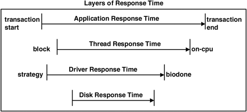
The sequence of events in Figure 4.4 is accurate for raw devices but is less meaningful for block devices. Reads on block devices often trigger read-ahead, which at times drives the disks asynchronously to the application reads; and writes often return from the cache and are later flushed to disk.
To understand the performance effect of response times purely from an application perspective, focus on thread and application response times and treat the disk I/O system as a black box. This leaves application latency as the most useful measurement, as discussed in Section 5.3.
The DTraceToolkit is a free collection of DTrace-based tools, some of which analyze disk behavior. We previously demonstrated cut-down versions of two of its scripts, bitesize.d and seeksize.d. Two of the most popular are iotop and iosnoop.
iotop uses DTrace to print disk I/O summaries by process, for details such as size (bytes) and disk I/O times. The following demonstrates the default output of iotop, which prints size summaries and refreshes the screen every five seconds.
# ./iotop
2006 Feb 13 13:38:21,  load: 0.35,  disk_r:  56615 Kb,  disk_w:    637 Kb

  UID    PID   PPID CMD              DEVICE  MAJ MIN D            BYTES
    0  27732  27703 find             cmdk0   102   0 R            38912
    0      0      0 sched            cmdk5   102 320 W           150016
    0      0      0 sched            cmdk2   102 128 W           167424
    0      0      0 sched            cmdk3   102 192 W           167424
    0      0      0 sched            cmdk4   102 256 W           167424
    0  27733  27703 bart             cmdk0   102   0 R         57897984
...
In the above output, the bart process read approximately 57 Mbytes from disk. Disk I/O time summaries can also be printed with -o, which uses the adaptive disk-response-time algorithm previously discussed. Here we demonstrate this with an interval of ten seconds.
# ./iotop -o 10
2006 Feb 13 13:39:19,  load: 0.38,  disk_r:  74885 Kb,  disk_w:   1345 Kb

  UID    PID   PPID CMD              DEVICE  MAJ MIN D         DISKTIME
    1    418      1 nfsd             cmdk3   102 192 W              362
    1    418      1 nfsd             cmdk4   102 256 W              382
    1    418      1 nfsd             cmdk5   102 320 W              460
    1    418      1 nfsd             cmdk2   102 128 W              534
    0      0      0 sched            cmdk5   102 320 W            20643
    0      0      0 sched            cmdk3   102 192 W            25500
    0      0      0 sched            cmdk4   102 256 W            31024
    0      0      0 sched            cmdk2   102 128 W            35166
    0  27732  27703 find             cmdk0   102   0 R           722951
    0  27733  27703 bart             cmdk0   102   0 R          8858818
Note that iotop prints totals, not per second values. In this example, we read 74, 885 Mbytes from disk during those ten seconds (disk_r), with the top process bart (PID 27733) consuming 8.8 seconds of disk time. For this ten-second interval, 8.8 seconds equates to a utilization value of 88%.
iotop can print %I/O utilization with the -P option; this percentage is based on 1000 ms of disk response time per second. The -C option can also be used to prevent the screen from being cleared and to instead provide a rolling output.
# ./iotop -CP 1
...
2006 Feb 13 13:40:34,  load: 0.36,  disk_r:   2350 Kb,  disk_w:   1026 Kb

  UID    PID   PPID CMD              DEVICE  MAJ MIN D   %I/O
    0      0      0 sched            cmdk0   102   0 R      0
    0      3      0 fsflush          cmdk0   102   0 W      1
    0  27743  27742 dtrace           cmdk0   102   0 R      2
    0      3      0 fsflush          cmdk0   102   0 R      8
    0      0      0 sched            cmdk0   102   0 W     14
    0  27732  27703 find             cmdk0   102   0 R     19
    0  27733  27703 bart             cmdk0   102   0 R     42
...
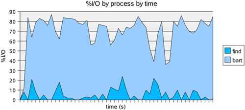
Figure 4.5 plots %I/O as find and bart read through /usr. This time bart causes heavier %I/O because there are bigger files to read and fewer directories for find to traverse.
Other options for iotop can be listed with -h (this is version 0.75):
# ./iotop -h
USAGE: iotop [-C] [-D|-o|-P] [-j|-Z] [-d device] [-f filename]
             [-m mount_point] [-t top] [interval [count]]

                -C      # don't clear the screen
                -D      # print delta times, elapsed, us
                -j      # print project ID
                -o      # print disk delta times, us
                -P      # print %I/O (disk delta times)
                -Z      # print zone ID
                -d device       # instance name to snoop
                -f filename     # snoop this file only
                -m mount_point  # this FS only
                -t top          # print top number only
   eg,
        iotop         # default output, 5 second samples
        iotop 1       # 1 second samples
        iotop -P      # print %I/O (time based)
        iotop -m /    # snoop events on filesystem / only
        iotop -t 20   # print top 20 lines only
        iotop -C 5 12 # print 12 x 5 second samples
These options including printing Zone and Project details.
iosnoop uses DTrace to monitor disk events in real time. The default output prints details such as PID, block address, and size. In the following example, a grep process reads several files from the /etc/default directory.
# ./iosnoop
  UID   PID D    BLOCK   SIZE       COMM PATHNAME
    0  1570 R   172636   2048       grep /etc/default/autofs
    0  1570 R   102578   1024       grep /etc/default/cron
    0  1570 R   102580   1024       grep /etc/default/devfsadm
    0  1570 R   108310   4096       grep /etc/default/dhcpagent
    0  1570 R   102582   1024       grep /etc/default/fs
    0  1570 R   169070   1024       grep /etc/default/ftp
    0  1570 R   108322   2048       grep /etc/default/inetinit
    0  1570 R   108318   1024       grep /etc/default/ipsec
    0  1570 R   102584   2048       grep /etc/default/kbd
    0  1570 R   102588   1024       grep /etc/default/keyserv
    0  1570 R   973440   8192       grep /etc/default/lu
...
The output is printed as the disk events complete.
To see a list of available options for iosnoop, use the -h option. The options include -o to print disk I/O time, using the adaptive disk-response-time algorithm previously discussed. The following is from iosnoop version 1.55.
# ./iosnoop -h
USAGE: iosnoop [-a|-A|-DeghiNostv] [-d device] [-f filename]
               [-m mount_point] [-n name] [-p PID]
       iosnoop          # default output
                -a      # print all data (mostly)
                -A      # dump all data, space delimited
                -D      # print time delta, us (elapsed)
                -e      # print device name
                -g      # print command arguments
                -i      # print device instance
                -N      # print major and minor numbers
                -o      # print disk delta time, us
                -s      # print start time, us
                -t      # print completion time, us
                -v      # print completion time, string
                -d device       # instance name to snoop
                -f filename     # snoop this file only
                -m mount_point  # this FS only
                -n name         # this process name only
                -p PID          # this PID only
   eg,
        iosnoop -v      # human readable timestamps
        iosnoop -N      # print major and minor numbers
        iosnoop -m /    # snoop events on filesystem / only
The block addresses printed are relative to the disk slice, so what may appear to be similar block addresses may in fact be on different slices or disks. The -N option can help ensure that we are examining the same slice since it prints major and minor numbers on which we can be match.
Using the -t option for iosnoop prints the disk completion time in microseconds. In combination with -N, we can use this data to plot disk events for a process on one slice. Here we fetch the data for the find command, which contains the time (microseconds since boot) and block address. These are our X and Y coordinates. We check that we remain on the same slice (major and minor numbers) and then generate an X/Y plot.
# ./iosnoop -tN
TIME           MAJ MIN   UID   PID D    BLOCK   SIZE       COMM PATHNAME
1175384556358  102   0     0 27703 W  3932432   4096        ksh /root/.sh_history
1175384556572  102   0     0 27703 W     3826    512        ksh <none>
1175384565841  102   0     0 27849 R   198700   1024       find /usr/dt
1175384578103  102   0     0 27849 R   770288   3072       find /usr/dt/bin
1175384582354  102   0     0 27849 R   690320   8192       find <none>
1175384582817  102   0     0 27849 R   690336   8192       find <none>
1175384586787  102   0     0 27849 R   777984   2048       find /usr/dt/lib
1175384594313  102   0     0 27849 R   733880   1024       find /usr/dt/lib/amd64
...
We ran a find / command to generate random disk activity; the results are shown in Figure 4.6. As the disk heads seek to different block addresses, the position of the heads is plotted in red.
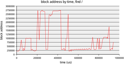
Are we really looking at disk head seek patterns? Not exactly. What we are looking at are block addresses for biodone functions from the block I/O driver. We aren’t using some X-ray vision to look at the heads themselves.
Now, if this is a simple disk device, then the block address probably relates to the disk head location.[12] But if this is a virtual device, say, a storage array, then block addresses could map to anything, depending on the storage layout. However, we could at least say that a large jump in block address probably means a seek at some point (although storage arrays will cache).
The block addresses do help us visualize the pattern of completed disk activity. But remember that “completed” means the block I/O driver thinks that the I/O event completed.
Previously, we discussed concurrent disk activity and included a plot (Figure 4.2) to help us understand how these events may occur. Since DTrace can easily trace concurrent disk activity, we can include a plot of actual activity. The following DTrace script provides input for a spreadsheet. We match on a device by its major and minor numbers, then print timestamps as the first column and block addresses for strategy and biodone events in the remaining columns.
#!/usr/sbin/dtrace -s
#pragma D option quiet

io:genunix::start
/args[1]->dev_major == 102 && args[1]->dev_minor == 0/
{
        printf("%d,%d,
", timestamp/1000, args[0]->b_blkno);
}
io:genunix::done
/args[1]->dev_major == 102 && args[1]->dev_minor == 0/
{
        printf("%d,,%d
", timestamp/1000, args[0]->b_blkno);
}
The output of the DTrace script was plotted as Figure 4.7, with timestamps as X-coordinates.
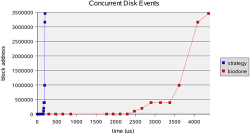
Initially, we see many quick strategies between 0 and 200 µs, ending in almost a vertical line. This is then followed by slower biodones as the disk catches up at mechanical speeds.
TazTool[13] was a GUI disk-analysis tool that used TNF tracing to monitor disk events. It was most notable for its unique disk-activity visualization, which made identifying disk access patterns trivial. This visualization included long-term patterns that would normally be difficult to identify from screenfuls of text.
This visualization technique is returning with the development of a DTrace version of taztool: DTraceTazTool. A screenshot of this tool is shown in Figure 4.8.
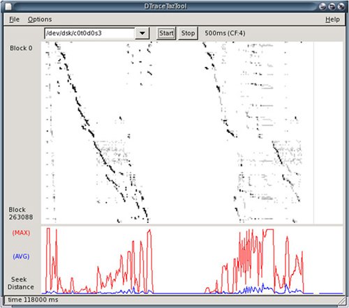
The first section of the plot measures a ufsdump of a file system, and the second measures a tar archive of the same file system, both times freshly mounted. We can see that the ufsdump command caused heavier sequential access (represented by dark stripes in the top graph and smaller seeks in the bottom graph) than did the tar command.
It is interesting to note that when the ufsdump command begins, disk activity can be seen to span the entire slice—ufsdump doing its passes.
[1] iostat -D prints the same statistic and calls it “util” or “percentage disk utilization.”
[2] Many of these were actually added in Solaris 2.6. The Solaris 2.5 Synopsis for iostat was /
usr/bin/iostat [ -cdDItx ] [ -l n ] [ disk . . . ] [ interval [ count ] ]
[3] If you would like to cling to the original single-line summaries of iostat, try iostat -cnDl99 1. Make your screen wide if you have many disks. Add a -P for some real entertainment.
[4] A throwback to when ttys were real teletypes, and service times were real service times.
[5] “DISK_NEW” for iostat means sometime before Solaris 2.5.
[6] See cmd/stat/common/acquire.c: insert_into() scans a list of I/O devices, calling iodev_cmp() to decide placement. iodev_cmp() initially groups in the following order: controllers, disks/partitions, tapes, NFS, I/O paths, unknown. strcmp() is then used for alphabetical sorting.
[7] We know this from watching iostat while a simple dd test runs: dd if =/dev/rdsk/c0t0d0s0 of =/dev/null bs =128K.
[8] Pending bug 6302763.
[9] Some people do automate iostat to run at regular intervals and log the output. Having this sort of comparative data on hand during a crisis can be invaluable.
[10] It’s possible that sar was written before the kilobytes unit was conventional.
[11] Solaris 10 does ship with StarOffice™ 7, which can plot interactively.
[12] Even “simple” disks these days map addresses in firmware to an internal optimized layout; all we know is the image of the disk that its firmware presents. The classic example here is sector zoning, as discussed in Section 4.4.
[13] See http://www.solarisinternals.com/si/tools/taz for more information.