
Chapter 7. Oracle Kernel Timings
Regardless of whether you access the Oracle kernel’s timing
statistics through extended SQL trace data, V$ fixed views, or even by hacking directly
into the Oracle shared memory segment beneath those V$ fixed views, the time statistics you’re
accessing were obtained using a simple set of operating system function
calls. Regardless of which interface you use to access them, those
timing statistics are subject to the limitations inherent in the
operating system timers that were used to produce them. This chapter
explains those limitations and describes their true impact upon your
work.
Operating System Process Management
From the perspective of your system’s host operating system, the Oracle kernel is just an application. There’s nothing mystical about how it works; it’s just a huge, extremely impressive C program. To gain a full appreciation for the operational timing data that the Oracle kernel reveals, you need to understand a little bit about the services an operating system provides to the Oracle kernel.
In this section, I am going to focus my descriptions on the behavior of operating systems derived from Unix. If your operating system is a Unix derivative like Linux, Sun Solaris, HP-UX, IBM AIX, or Tru64, then the explanations you will see here will closely resemble the behavior of your system. You should find the descriptions in this section relevant even if you are studying a Microsoft Windows system. If your operating system is not listed here, then I suggest that you augment the descriptions in this section with the appropriate operating system internals documentation for your system.
The Design of the Unix Operating System, written by Maurice Bach, contains what is still my very favorite tool for describing what a process “does” in the context of a modern operating system. Bach’s Figure 2-6, entitled “Process States and Transitions” [Bach 1986 (31)], serves as my starting point. I have reproduced it here as Figure 7-1. In this diagram, each node (rectangle) represents a state that a process can take on in the operating system. Each edge (directed line) represents a transition from one state to another. Think of states as nouns and transitions as verbs that motivate the passage of a process from one state to the next.
![This simplified process state diagram illustrates the principal states that a process can assume in most modern time-sharing operating systems [Bach (1986) 31]](http://imgdetail.ebookreading.net/data/2/059600527X/059600527X__optimizing-oracle-performance__059600527X__httpatomoreillycomsourceoreillyimages2233676.png)
Most Oracle kernel processes spend most of their time in the user running state, also called user mode. Parsing SQL, sorting rows, reading blocks in the buffer cache, and converting data types are common operations that Oracle executes in user mode. There are two events that can cause a process to transition from the user running state to the kernel running state (also called kernel mode). It is important for you to understand both transitions from user mode to kernel mode. Let’s follow each one in more detail.
The sys call Transition
When a process in user mode makes an operating system
call (a sys call), it transitions to kernel
mode. read and select are two typical system calls. Once
in kernel mode, a process is endowed with special privileges that
allow it to manipulate low-level hardware components and arbitrary
memory locations. In kernel mode, a process is able, for example, to
manipulate I/O devices like sockets and disk drives [Bovet and
Cesati (2001) 8].
Many types of system call can be expected to wait on a device
for many, many CPU cycles. For example, a read call of a disk subsystem today
typically consumes time on the order of a few milliseconds. Many
CPUs today can execute millions of instructions in the time it takes
to execute one physical disk I/O operation. So during a single read
call, enough time to perform on the order of a million CPU
instructions will elapse. Designers of efficient read system calls of course realize this
and design their code in a manner that allows another process to use
the CPU while the reading process
waits.
Imagine, for example, an Oracle kernel process executing some
kind of read system call to
obtain a block of Oracle data from a disk. After issuing a request
from an expectedly “slow” device, the kernel code in the read system call will transition its
calling process into the sleep
state, where that process will await an interrupt signaling that the
I/O operation is complete. This polite yielding of the CPU allows
another ready to run process to
consume the CPU capacity that the reading process would have been unable to
use anyway.
When the I/O device signals that the asleep process’s I/O operation is ready
for further processing, the process is “awoken,” which is to say
that it transitions to ready to
run state. When the process becomes ready to run, it
becomes eligible for scheduling. When the scheduler again chooses
the process for execution, the process is returned to kernel running state, where the remaining
kernel mode code path of the read
call is executed (for example, the data transfer of the content
obtained from the I/O channel into memory). The final instruction in
the read subroutine returns
control to the calling program (our Oracle kernel process), which is
to say that the process transitions back into user running state. In this state, the
Oracle kernel process continues consuming user-mode CPU until it
next receives an interrupt or makes a system call.
The interrupt Transition
The second path through the operating system process state diagram is motivated by an interrupt. An interrupt is a mechanism through which a device such as an I/O peripheral or the system clock can interrupt the CPU asynchronously [Bach (1986) 16]. I’ve already described why an I/O peripheral might interrupt a process. Most systems are configured so that the system clock generates an interrupt every 1/100th of a second (that is, once per centisecond). Upon receipt of a clock interrupt, each process on the system in user running state saves its context (a frozen image of what the process was doing) and executes the operating system scheduler subroutine. The scheduler determines whether to allow the process to continue running or to preempt the process.
Preemption essentially sends a process directly from kernel running state to ready to run state, clearing the way for some other ready to run process to return to user running state [Bach (1986) 148]. This is how most modern operating systems implement time-sharing. Any process in ready to run state is subject to treatment that is identical to what I have described previously. The process becomes eligible for scheduling, and so on. Your understanding of preemptions motivated by clock interrupts will become particularly important later in this chapter when I describe one of the most important causes of “missing data” in an Oracle trace file.
Other States and Transitions
I have already alluded to the existence of a more complicated process state transition diagram than I’ve shown in Figure 7-1. Indeed, after discussing the four process states and seven of the transitions depicted in Figure 7-1, Bach later in his book reveals a more complete process state transition diagram [Bach (1986) 148]. The more complicated diagram details the actions undertaken during transitions such as preempting, swapping, forking, and even the creation of zombie processes. If you run applications on Unix systems, I strongly encourage you to add Bach’s book to your library.
For the purposes of the remainder of this chapter, however, Figure 7-1 is all you need. I hope you will agree that it is easy to learn the precise definitions of Oracle timing statistics by considering them in terms of the process states shown in Figure 7-1.
Oracle Kernel Timings
The Oracle kernel publishes only a few different types of timing information. Extended SQL trace output contains four important ones. You can see all four on the following two lines, generated by an Oracle release 9.0.1.2.0 kernel a Solaris 5.6 system:
WAIT #34: nam='db file sequential read'ela= 14118p1=52 p2=2755 p3=1 FETCH #34:c=0,e=15656,p=1,cr=6,cu=0,mis=0,r=1,dep=3,og=4,tim=1017039276349760
The two adjacent lines of trace data shown here describe a single fetch database call. The timing statistics in these lines are the following:
ela= 14118The Oracle kernel consumed an elapsed time of 14,118 microseconds (or μs, where 1 μs = 0.000 001 seconds) executing a system call denoted
db file sequential read.c=0The Oracle kernel reports that a fetch database call consumed 0 μs of total CPU capacity.
e=15656The kernel reports that the fetch consumed 15,656 μs of elapsed time.
tim=1017039276349760The system time when the fetch concluded was 1,017,039,276,349,760 (expressed in microseconds elapsed since midnight UTC 1 January 1970).
The total elapsed duration of the fetch includes both the call’s total CPU capacity consumption and any time that the fetch has consumed during the execution of Oracle wait events. The statistics in my two lines of trace data are related through the approximation:
| e ≈ c + ela |
In this case, the approximation is pretty good on a human scale: 15656 ≈ 0 + 14118, which is accurate to within 0.001538 seconds.
A single database call (such as a parse, execute, or fetch) emits only one database call line
(such as PARSE, EXEC, or FETCH) to the trace data (notwithstanding
the recursive database calls that a single
database call can motivate). However, a single database call may emit
several WAIT lines representing
system calls for each cursor action line. For example, the following
trace file excerpt shows 6,288 db file
sequential read calls executed by a single fetch:
WAIT #44: nam='db file sequential read' ela= 15147 p1=25 p2=24801 p3=1
...
6,284 similar WAIT lines are omitted here for clarity

...
WAIT #44: nam='db file sequential read' ela= 105 p1=25 p2=149042 p3=1
WAIT #44: nam='db file sequential read' ela= 18831 p1=5 p2=115263 p3=1
WAIT #44: nam='db file sequential read' ela= 114 p1=58 p2=58789 p3=1
FETCH #44:c=7000000,e=23700217,p=6371,cr=148148,cu=0,mis=0,r=1,dep=1,og=4,
tim=1017039304454213
So the true relationship that binds the values of c, e, and
ela for a given database call must
refer to the sum of ela values that were produced within the
context of a given database call:
This approximation is the basis for all response time measurement in the Oracle kernel.
How Software Measures Itself
Finding out how the Oracle kernel measures itself is not
a terribly difficult task. This section is based on studies of
Oracle8i and Oracle9i kernels running on Linux systems. The
Oracle software for your host operating system might use different
system calls than our system uses. To find out, you should see how
your Oracle system behaves by using a software
tool that traces system calls for a specified process. For example,
Linux provides a tool called strace
to trace system calls. Other operating systems use different names for
the tool. There is truss for Sun
Solaris (truss is actually the
original system call tracing tool for Unix), sctrace for IBM AIX, tusc for HP-UX, and strace for Microsoft Windows. I shall use
the Linux name strace to refer
generically to the collection of tools that trace system
calls.
Tip
At the time of this writing, it is possible to find strace tools for several operating systems
at http://www.pugcentral.org/howto/truss.htm.
The strace tool is easy to
use. For example, you can observe directly what the Oracle kernel is
doing, right when each action takes place, by executing a command like
the following:
$ strace -p 12417
read(7,
In this example, strace shows
that a Linux program with process ID 12417 (which happens to have been
an Oracle kernel process on my system) has issued a read call and is awaiting fulfillment of
that call (hence the absence of the right parenthesis in the output
shown here).
It is especially instructive to view strace output and Oracle SQL trace output
simultaneously in two windows, so that you can observe exactly
when lines are emitted to both output streams.
The write calls that the Oracle
kernel uses to emit its trace data of course appear in the strace output exactly when you would expect
them to. The appearance of these calls makes it easy to understand
when Oracle kernel actions produce trace data. In
Oracle9i for Linux (and Oracle9i for some other operating systems), it is
especially easy to correlate strace
output and SQL trace output, because values returned by gettimeofday appear directly in the trace
file as tim values. By using
strace and SQL trace simultaneously
in this manner, you can positively confirm or refute whether your
Oracle kernel behaves like the pseudocode that you will see in the
following sections.
Tip
Using strace will introduce
significant measurement intrusion effect into
the performance of the program you’re tracing. I discuss the
performance effects of measurement intrusion later in this
chapter.
Elapsed Time
The Oracle kernel derives all of its timing statistics from the results of system calls issued upon the host operating system. Example 7-1 shows how a program like the Oracle kernel computes the durations of its own actions.
t0 = gettimeofday;   # mark the time immediately before doing something
do_something;
t1 = gettimeofday;   # mark the time immediately after doing it
t = t1 - t0;         # t is the approximate duration of do_something
The gettimeofday function
is an operating system call found on POSIX-compliant systems. You
can learn by viewing your operating system’s documentation that
gettimeofday provides a C
language data structure to its caller that contains the number of
seconds and microseconds that have elapsed since the Epoch, which is
00:00:00 Coordinated Universal Time (UTC), January 1, 1970.
Note
Documentation for such system calls is usually available
with your operating system. For example, on Unix systems, you can
view the gettimeofday
documentation by typing man
gettimeofday at the Unix prompt. Or you can visit http://www.unix-systems.org/single_unix_specification/
to view the POSIX definition.
Note that in my pseudocode, I’ve hidden many mechanical
details that I find distracting. For example, gettimeofday doesn’t really return a
time; it returns 0 for success and -1 for failure. It writes the
“returned” time as a two-element structure (a seconds part and a microseconds part) in a location
referenced by the caller’s first argument in the gettimeofday call. I believe that
showing all this detail in my pseudocode would serve only to
complicate my descriptions unnecessarily.
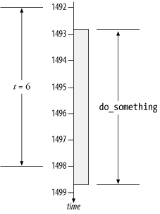
Imagine the execution of Example 7-1 on a timeline, as
shown in Figure 7-2.
In the drawing, the value of the gettimeofday clock is t 0 = 1492 when a
function called do_something
begins. The value of the gettimeofday clock is t 1 = 1498 when
do_something ends. Thus the
measured duration of do_something
is t = t 1 - t 0 = 6 clock
ticks.
Tip
I’ve used the time values 1492 through 1499 to keep our
discussion simple. These values of course do not resemble the
actual second and microsecond values that gettimeofday would return in the
twenty-first century. Consider the values I’ll discuss in this
book to be just the final few digits of an actual clock.
The Oracle kernel reports on two types of elapsed duration:
the e statistic denotes the
elapsed duration of a single database call, and the ela statistic denotes the elapsed duration
of an instrumented sequence of instructions (often a system call)
executed by an Oracle kernel process. The kernel performs these
computations by executing code that is structured roughly like the
pseudocode shown in Example
7-2. Notice that the kernel uses the method shown in Example 7-1 as the basic
building block for constructing the e and ela metrics.
procedure dbcall {
    e0 = gettimeofday;      # mark the wall time
    ...                     # execute the db call (may call wevent)
    e1 = gettimeofday;      # mark the wall time
    e = e1 - e0;            # elapsed duration of dbcall
    print(TRC, ...);        # emit PARSE, EXEC, FETCH, etc. line
}

procedure wevent {
    ela0 = gettimeofday;    # mark the wall time
    ...                     # execute the wait event here
    ela1 = gettimeofday;    # mark the wall time
    ela = ela1 - ela0;      # ela is the duration of the wait event
    print(TRC, "WAIT...");  # emit WAIT line
}
CPU Consumption
The Oracle kernel reports not only the elapsed
duration e for each database call
and ela for each system call, but
also the amount of total CPU capacity c consumed by each database call. In the
context of the process state transition diagram shown in Figure 7-1, the c statistic is defined as the approximate
amount of time that a process has spent in the following
states:
| user running |
| kernel running |
On POSIX-compliant operating systems, the Oracle kernel
obtains CPU usage information from a function called getrusage on Linux and many other
operating systems, or a similar function called times on HP-UX and a few other systems.
Although the specifications of these two system calls vary
significantly, I will use the name getrusage to refer generically to either
function. Each function provides its caller with a variety of
statistics about a process, including data structures representing
the following four characteristics:
Approximate time spent by the process in user running state
Approximate time spent by the process in kernel running state
Approximate time spent by the process’s children in user running state
Approximate time spent by the process’s children in kernel running state
Each of these amounts is expressed in microseconds, regardless of whether the data are accurate to that degree of precision.
Tip
You’ll see shortly that, although by POSIX standard,
getrusage returns information
expressed in microseconds, rarely does the information contain
detail at sub-centisecond resolution.
The Oracle kernel performs c, e,
and ela computations by executing
code that is structured roughly like the pseudocode shown in Example 7-3. Notice that this
example builds upon Example
7-2 by including executions of the getrusage system call and the subsequent
manipulation of the results. In a method analogous to the gettimeofday calculations, the Oracle
kernel marks the amount of user-mode CPU time consumed by the
process at the beginning of the database call, and then again at the
end. The difference between the two marks (c0 and c1) is the approximate amount of CPU
capacity that was consumed by the database call. Shortly I’ll fill
you in on exactly how approximate the amount is.
procedure dbcall {
    e0 = gettimeofday;          # mark the wall time
    c0 = getrusage;             # obtain resource usage statistics
    ...                         # execute the db call (may call wevent)
    c1 = getrusage;             # obtain resource usage statistics
    e1 = gettimeofday;          # mark the wall time
    e = e1 - e0;                # elapsed duration of dbcall
    c = (c1.utime + c1.stime)
      - (c0.utime + c0.stime);  # total CPU time consumed by dbcall
    print(TRC, ...);            # emit PARSE, EXEC, FETCH, etc. line
}

procedure wevent {
    ela0 = gettimeofday;        # mark the wall time
    ...                         # execute the wait event here
    ela1 = gettimeofday;        # mark the wall time
    ela = ela1 - ela0;          # ela is the duration of the wait event
    print(TRC, "WAIT...");      # emit WAIT line
}
Unaccounted-for Time
Virtually every trace file you’ll ever analyze will have some mismatch between actual response time and the amount of time that the Oracle kernel accounts for in its trace file. Sometimes there will be an under-counting of time, and sometimes there will be an over-counting of time. For reasons you’ll understand shortly, under-counting is more common than over-counting. In this book, I refer to both situations as unaccounted-for time. When there’s missing time, there is a positive unaccounted-for duration. When there is an over-counting of time, there is a negative unaccounted-for duration. Unaccounted-for time in Oracle trace files can be caused by five distinct phenomena:
Measurement intrusion effect
CPU consumption double-counting
Quantization error
Time spent not executing
Un-instrumented Oracle kernel code
I’ll discuss each of these contributors of unaccounted-for time in the following sections.
Measurement Intrusion Effect
Any software application that attempts to measure the elapsed durations of its own subroutines is susceptible to a type of error called measurement intrusion effect [Malony et al. (1992)]. Measurement intrusion effect is a type of error that occurs because the execution duration of a measured subroutine is different from the execution duration of the subroutine when it is not being measured. In recent years, I have not had reason to suspect that measurement intrusion effect has meaningfully influenced any Oracle response time measurement I’ve analyzed. However, understanding the effect has helped me fend off illegitimate arguments against the reliability of Oracle operational timing data.
To understand measurement intrusion, imagine the following problem. You have a program called U, which looks like this:
program U {
    # uninstrumented
    do_something;
}
Your goal is to find out how much time is consumed by the
subroutine called do_something. So
you instrument your program U,
resulting in a new program called I:
program I {
    # instrumented
    e0 = gettimeofday;  # instrumentation
    do_something;
    e1 = gettimeofday;  # instrumentation
    printf("e=%.6f sec
", (e1-e0)/1E6);
}
You would expect this new program I to print the execution duration of
do_something. But the value it
prints is only an approximation of do_something’s runtime duration. The value
being printed, e1 - e0 converted to seconds, contains not just
the duration of do_something, but
the duration of one gettimeofday
call as well. The picture in Figure 7-3 shows why.

The impact of measurement intrusion effect upon program U is the following:
Execution time of I includes two
gettimeofdaycode paths more than the execution time of U.The measured duration of
do_somethingin I includes one fullgettimeofdaycode path more thando_somethingactually consumes.
This impact is minimal for applications in which the duration of
one gettimeofday call is small
relative to the duration of whatever do_something-like subroutine you are
measuring. However, on systems with inefficient gettimeofday implementations (I believe that
HP-UX versions prior to release 10 could be characterized this way),
the effect could be meaningful.
Measurement intrusion effect is a type of systematic
error. A systematic error is the result of an experimental
“mistake” that is consistent across measurements [Lilja (2000)]. The
consistency of measurement intrusion makes it possible to compute its
influence upon your data. For example, to quantify the Oracle kernel’s
measurement intrusion effect introduced by gettimeofday calls, you need two pieces of
data:
The number of timer calls that the Oracle kernel makes for a given operation.
The expected duration of a single timer call.
Once you know the frequency and average duration of your Oracle kernel’s timer calls, you have everything you need to quantify their measurement intrusion effect. Measurement intrusion is probably one reason for the missing time that you will encounter when performing an Oracle9i clock-walk (Chapter 5).
Finding these two pieces of data is not difficult. You can use
the strace tool for your platform
to find out how many timer calls your Oracle kernel makes for a given
set of database operations. To compute the expected duration of one
timer call, you can use a program like the one shown in Example 7-4. This code measures
the distance between adjacent gettimeofday calls and then computes their
average duration over a sample size of your choosing.
#!/usr/bin/perl # $Header: /home/cvs/cvm-book1/measurement�40intrusion/mef.pl,v 1.4 2003/03/19 04:38:48 cvm Exp $ # Cary Millsap ([email protected]) # Copyright (c) 2003 by Hotsos Enterprises, Ltd. All rights reserved. use strict; use warnings; use Time::HiRes qw(gettimeofday); sub fnum($;$$) { # return string representation of numeric value in # %.${precision}f format with specified separators my ($text, $precision, $separator) = @_; $precision = 0 unless defined $precision; $separator = "," unless defined $separator; $text = reverse sprintf "%.${precision}f", $text; $text =~ s/(ddd)(?=d)(?!d*.)/$1$separator/g; return scalar reverse $text; } my ($min, $max) = (100, 0); my $sum = 0; print "How many iterations? "; my $n = <>; print "Enter 'y' if you want to see all the data: "; my $all = <>; for (1 .. $n) { my ($s0, $m0) = gettimeofday; my ($s1, $m1) = gettimeofday; my $sec = ($s1 - $s0) + ($m1 - $m0)/1E6; printf "%0.6f ", $sec if $all =~ /y/i; $min = $sec if $sec < $min; $max = $sec if $sec > $max; $sum += $sec; } printf "gettimeofday latency for %s samples ", fnum($n); printf " %0.6f seconds minimum ", $min; printf " %0.6f seconds maximum ", $max; printf " %0.9f seconds average ", $sum/$n;
On my Linux system used for research (800MHz Intel Pentium),
this code reveals typical gettimeofday latencies of about 2 μs:
Linux$mefHow many iterations?1000000Enter 'y' if you want to see all the data:ngettimeofday latency for 1,000,000 samples 0.000001 seconds minimum 0.000376 seconds maximum 0.000002269 seconds average
Measurement intrusion effect depends greatly upon operating
system implementation. For example, on my Microsoft Windows 2000
laptop computer (also 800MHz Intel Pentium), gettimeofday causes more than 2.5 times as
much measurement intrusion effect as our Linux server, with an average
of almost 6 μs:
Win2k$perl mef.plHow many iterations?1000000Enter 'y' if you want to see all the data:ngettimeofday latency for 1,000,000 samples 0.000000 seconds minimum 0.040000 seconds maximum 0.000005740 seconds average
By experimenting with system calls in this manner, you can begin to understand some of the constraints under which the kernel developers at Oracle Corporation must work. Measurement intrusion effect is why developers tend to create timing instrumentation only for events whose durations are long relative to the duration of the measurement intrusion. The tradeoff is to provide valuable timing information without debilitating the performance of the application being measured.
CPU Consumption Double-Counting
Another inaccuracy in the relationship:
is an inherent double-counting of CPU time in the right-hand
side of the approximation. The Oracle kernel definition of the
c statistic is all time spent in
user running and kernel running states. Each ela statistic contains all time spent within
an instrumented sequence of Oracle kernel instructions. When the
instrumented sequence of instructions causes consumption of CPU
capacity, that consumption is double-counted.
For example, imagine an Oracle database call that performs a
disk read, such as the one shown in Figure 7-4. In this drawing, a
database call begins its execution at time e 0. For the
duration labeled A, the call
consumes CPU capacity in the user running state. At time ela 0, the Oracle
kernel process issues the gettimeofday call that precedes the
execution of an Oracle wait event. Depending upon the operating
system, the execution of the gettimeofday system call puts the Oracle
kernel process into kernel running state for a few microseconds before
retuning the process to user running state.
Tip
Some Linux kernels allow the gettimeofday system call to execute
entirely in user running state, resulting in a significant
performance improvement (for one example, see http://www-124.ibm.com/linux/patches/?patch_id=597).
After some more CPU consumption in user running state for the duration labeled B, the process transitions into kernel running state for the duration labeled C. At the conclusion of duration C, the kernel process transitions to the asleep state and awaits the result of the request from the disk.
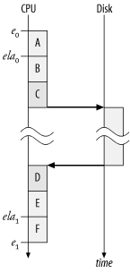
Upon completion of the request, the disk sends an interrupt that motivates the wakeup of the Oracle kernel process, which then transitions to the ready to run state. In Figure 7-4, the CPU is idle at this point in time, and the process is immediately scheduled and thus transitioned to kernel running state. While executing in this state, the Oracle process then wraps up the details of the disk I/O call, such as the copying of the data from the I/O channel to the Oracle process’s user-addressable memory, which consumes the duration labeled D.
Finally at the end of duration D, the disk read call returns, and the
Oracle process transitions to user running state for the duration
labeled E. At time ela 1, the Oracle
process marks the end of the disk read with a gettimeofday call. The Oracle process then
proceeds to execute the remaining instructions (also in user running
state) that are required to complete the database call. Finally, at
time e 1,
the database call processing is complete.
As the result of these actions, the Oracle kernel will produce the following statistics for the database call:
e = e 1 - e 0 |
ela = ela 1 - ela 0 = B + C + Disk + D + E |
c = A + B + C + D + E + F |
I shall describe, a little later, exactly how c is computed. The value that c will have is approximately the sum of the
durations A, B, C,
D, E, and F. At this point, it should be easy for you
to see where the double-counting occurs. Both ela and c
contain the durations B,
C, D, and E. The segments of CPU consumption that
have occurred within the confines of the wait event have been
double-counted.
How big of a problem is the double-counting? Fortunately, the
practical impact is usually negligible. Our experience with over a
thousand trace files at http://www.hotsos.com
indicates that the durations marked as B, C,
D, and E in Figure 7-4 are usually small.
It appears that most of the wait events instrumented in
Oracle8i and Oracle9i have response times (that is, ela values) that are dominated by durations
other than CPU consumption. In a few rare cases (I’ll show you one
shortly), the double-counting shows up in small sections of trace
data, but in the overall scheme of Oracle response time accounting,
the effect of CPU consumption double-counting
seems to be generally negligible.
Quantization Error
A few years ago, a friend argued that Oracle’s extended SQL trace capability was a performance diagnostic dead-end. His argument was that in an age of 1GHz CPUs, the one-centisecond resolution of the then-contemporary Oracle8i kernel was practically useless. However, in many hundreds of projects in the field, the extended SQL trace feature has performed with practically flawless reliability—even the “old one-centisecond stuff” from Oracle8i. The reliability of extended SQL trace is difficult to understand unless you understand the properties of measurement resolution and quantization error.
Measurement Resolution
When I was a kid, one of the everyday benefits of growing up in the Space Age was the advent of the digital alarm clock. Digital clocks are fantastically easy to read, even for little boys who don’t yet know how to “tell the time.” It’s hard to go wrong when you can see those big red numbers showing “7:29”. With an analog clock, a kid sometimes has a hard time knowing whether it’s five o’clock and seven o’clock, but the digital difference between 5 and 7 is unmistakable.
But there’s a problem with digital clocks. When you glance at a digital clock that shows “7:29”, how close is it to 7:30? The problem with digital clocks is that you can’t know. With a digital clock, you can’t tell whether it’s 7:29:00 or 7:29:59 or anything in-between. With an analog clock, even one without a second-hand, you can guess about fractions of minutes by looking at how close the minute hand is to the next minute.
All times measured on digital computers derive ultimately from interval timers, which behave like the good old digital clocks at our bedsides. An interval timer is a device that ticks at fixed time intervals. Times collected from interval timers can exhibit interesting idiosyncrasies. Before you can make reliable decisions based upon Oracle timing data, you need to understand the limitations of interval timers.
An interval timer’s resolution is the elapsed duration between adjacent clock ticks. Timer resolution is the inverse of timer frequency. So a timer that ticks at 1 GHz (approximately 109 ticks per second) has a resolution of approximately 1/109 seconds per tick, or about 1 nanosecond (ns) per tick. The larger a timer’s resolution, the less detail it can reveal about the duration of a measured event. But for some timers (especially ones involving software), making the resolution too small can increase system overhead so much that you alter the performance behavior of the event you’re trying to measure.
As a timing statistic passes upward from hardware through various layers of application software, each application layer can either degrade its resolution or leave its resolution unaltered. For example:
The resolution of the result of the
gettimeofdaysystem call, by POSIX standard, is one microsecond. However, many Intel Pentium CPUs contain a hardware time stamp counter that provides resolution of one nanosecond. The Linuxgettimeofdaycall, for example, converts a value from nanoseconds (10-9 seconds) to microseconds (10-6 seconds) by performing an integer division of the nanosecond value by 1,000, effectively discarding the final three digits of information.The resolution of the
estatistic on Oracle8i is one centisecond. However, most modern operating systems providegettimeofdayinformation with microsecond accuracy. The Oracle8i kernel converts a value from microseconds (10-6 seconds) to centiseconds (10-2 seconds) by performing an integer division of the microsecond value by 10,000, effectively discarding the final four digits of information [Wood (2003)].
Thus, each e and ela statistic emitted by an
Oracle8i kernel actually
represents a system characteristic whose actual value cannot be
known exactly, but which resides within a known range of values.
Such a range of values is shown in Table 7-1. For example,
the Oracle8i statistic e=2 can refer to any actual elapsed
duration e
a in the range:
| 2.000 0 cs < e a < 2.999 9 cs |
Definition of Quantization Error
Quantization error is the quantity E defined as the difference between an event’s actual duration e a and its measured duration e m . That is:
| E = e m - e a |
Let’s revisit the execution of Example 7-1 superimposed upon
a timeline, as shown in Figure 7-5. In this drawing,
each tick mark represents one clock tick on an interval timer like
the one provided by gettimeofday.
The value of the timer was t
0 = 1492 when do_something began. The value of the timer
was t 1
= 1498 when do_something ended.
Thus the measured duration of do_something was e m
= t
1 - t
0 = 6. However, if you physically measure the
length of the duration e
a in the drawing,
you’ll find that the actual duration of do_something is e a
= 5.875 ticks. You can confirm the actual duration by
literally measuring the height of e a
in the drawing, but it is not possible for an
application to “know” the value of e a
by using only the interval timer whose ticks are shown
in Figure 7-5. The
quantization error is E =
e
m - e a
= 0.125 ticks, or about 2.1 percent of the 5.875-tick
actual duration.

Now, consider the case when the duration of do_something is much closer to the timer
resolution, as shown in Figure 7-6. In the left-hand
case, the duration of do_something spans one clock tick, so it
has a measured duration of e
m = 1. However, the
event’s actual duration is only e a
= 0.25. (You can confirm this by measuring the actual
duration in the drawing.) The quantization error in this case is
E = 0.75, which is a whopping
300% of the 0.25-tick actual duration. In the right-hand case, the
execution of do_something spans
no clock ticks, so it has a measured duration of e m
= 0; however, its actual duration is e a
= 0.9375. The quantization error here is E = -0.9375, which is -100% of the
0.9375-tick actual duration.
To describe quantization error in plain language:
Any duration measured with an interval timer is accurate only to within one unit of timer resolution.
More formally, the difference between any two digital clock measurements is an elapsed duration with quantization error whose exact value cannot be known, but which ranges anywhere from almost -1 clock tick to almost +1 clock tick. If we use the notation r x to denote the resolution of some timer called x, then we have:
| x m - r x < x a < x m + r x |
The quantization error E inherent in any digital measurement is a uniformly distributed random variable (see Chapter 11) with range -r x < E < r x , where r x denotes the resolution of the interval timer.
Whenever you see an elapsed duration printed by the Oracle
kernel (or any other software), you must think in terms of the
measurement resolution. For example, if you see the statistic
e=4 in an Oracle8i trace file, you need to understand that
this statistic does not mean that the actual
elapsed duration of something was 4 cs. Rather, it means that
if the underlying timer resolution is 1 cs or
better, then the actual elapsed duration of something was between 3
cs and 5 cs. That is as much detail as you can know.
For small numbers of statistic values, this imprecision can lead to ironic results. For example, you can’t actually even make accurate comparisons of event durations for events whose measured durations are approximately equal. Figure 7-7 shows a few ironic cases. Imagine that the timer shown here is ticking in 1-centisecond intervals. This is behavior that is equivalent to the Oracle8i practice of truncating digits of timing precision past the 0.01-second position. Observe in this figure that event A consumed more actual elapsed duration than event B, but B has a longer measured duration; C took longer than D, but D has a longer measured duration. In general, any event with a measured duration of n + 1 may have an actual duration that is longer than, equal to, or even shorter than another event having a measured duration of n. You cannot know which relationship is true.

An interval timer can give accuracy only to ±1 clock tick, but in practical application, this restriction does not diminish the usefulness of interval timers. Positive and negative quantization errors tend to cancel each other over large samples. For example, the sum of the quantization errors in Figure 7-6 is:
| E 1 + E 2 = 0.75 + (-0.9375) = 0.1875 |
Even though the individual errors were proportionally large, the sum of the errors is a much smaller 16% of the sum of the two actual event durations. In a several hundred SQL trace files collected at http://www.hotsos.com from hundreds of different Oracle sites, we have found that positive and negative quantization errors throughout a trace file with hundreds of lines tend to cancel each other out. Errors commonly converge to magnitudes smaller than ±10% of the total response time measured in a trace file.
Complications in Measuring CPU Consumption
You may have noticed by now that your gettimeofday system call has much better
resolution than getrusage.
Although the pseudocode in Example 7-3 makes it look
like gettimeofday and getrusage do almost the same thing, the
two functions work in profoundly different ways. As a result, the
two functions produce results with profoundly different
accuracies.
How gettimeofday works
The operation of gettimeofday is much easier to
understand than the operation of getrusage. I’ll use Linux on Intel
Pentium processors as a model for explaining. As I mentioned
previously, the Intel Pentium processor has a hardware time stamp
counter (TSC) register that is updated on every hardware clock
tick. For example, a 1-GHz CPU will update its TSC approximately a
billion times per second [Bovet and Cesati (2001) 139-141]. By
counting the number of ticks that have occurred on the TSC since
the last time a user set the time with the date command, the Linux kernel can
determine how many clock ticks have elapsed since the Epoch. The
result returned by gettimeofday
is the result of truncating this figure to microsecond resolution
(to maintain the POSIX-compliant behavior of the gettimeofday function).
How getrusage works
There are two ways in which an operating system can account for how much time a process spends consuming user-mode or kernel-mode CPU capacity:
- Polling (sampling)
The operating system could be instrumented with extra code so that, at fixed intervals, each running process could update its own
rusagetable. At each interval, each running process could update its own CPU usage statistic with the estimate that it has consumed the entire interval’s worth of CPU capacity in whatever state the processes is presently executing in.- Event-based instrumentation
The operating system could be instrumented with extra code so that every time a process transitions to either user running or kernel running state, it could issue a high-resolution timer call. Every time a process transitions out of that state, it could issue another timer call and publish the microseconds’ worth of difference between the two calls to the process’
rusageaccounting structure.
Most operating systems use polling, at least by default. For example, Linux updates several attributes for each process, including the CPU capacity consumed thus far by the process, upon every clock interrupt [Bovet and Cesati (2001) 144-145]. Some operating systems do provide event-based instrumentation. Sun Solaris, for example, provides this feature under the name microstate accounting [Cockroft (1998)].
With microstate accounting, quantization error is limited to
one unit of timer resolution per state switch. With a
high-resolution timer (like gettimeofday), the total quantization
error on CPU statistics obtained from microstate accounting can be
quite small. However, the additional accuracy comes at the cost of
incrementally more measurement intrusion effect. With polling,
however, quantization error can be significantly worse, as you’ll
see in a moment.
Regardless of how the resource usage information is
obtained, an operating system makes this information available to
any process that wants it via a system call like getrusage. POSIX specifies that getrusage must use microseconds as its
unit of measure, but—for systems that obtain rusage information by polling—the true
resolution of the returned data depends upon the clock interrupt
frequency.
The clock interrupt frequency for most systems is 100 interrupts per second, or one interrupt every centisecond (operating systems texts often speak in terms of milliseconds; 1 cs = 10 ms = 0.010 s). The clock interrupt frequency is a configurable parameter on many systems, but most system managers leave it set to 100 interrupts per second. Asking a system to service interrupts more frequently than 100 times per second would give better time measurement resolution, but at the cost of degraded performance. Servicing interrupts even only ten times more frequently would intensify the kernel-mode CPU overhead consumed by the operating scheduler by a factor of ten. It’s generally not a good tradeoff.
If your operating system is POSIX-compliant, the following Perl program will reveal its operating system scheduler resolution [Chiesa (1996)]:
$cat clkres.pl#!/usr/bin/perl use strict; use warnings; use POSIX qw(sysconf _SC_CLK_TCK); my $freq = sysconf(_SC_CLK_TCK); my $f = log($freq) / log(10); printf "getrusage resolution %.${f}f seconds ", 1/$freq; $perl clkres.plgetrusage resolution: 0.01 seconds
With a 1-cs clock resolution, getrusage may return microsecond data,
but those microsecond values will never contain valid detail
smaller than 1/100th (0.01) of a
second.
The reason I’ve explained all this is that the quantization
error of the Oracle c statistic
is fundamentally different from the quantization error of an
e or ela statistic. Recall when I
wrote:
Any duration measured with an interval timer is accurate only to within one unit of timer resolution.
The problem with Oracle’s c statistic is that the statistic
returned by getrusage is
not really a duration. That is, a CPU
consumption “duration” returned by getrusage is not a statistic obtained by
taking the difference of a pair of interval timer measurements.
Rather:
On systems with microstate accounting activated, CPU consumption is computed as potentially very many short durations added together.
On systems that poll for
rusageinformation, CPU consumption is an estimate of duration obtained by a process of polling.
Hence, in either circumstance, the quantization error
inherent in an Oracle c
statistic can be much worse than just one
clock tick. The problem exists even on systems that use microstate
accounting. It’s worse on systems that don’t.
Figure 7-8 depicts an example of a standard polling-based situation in which the errors in user-mode CPU time attribution add up to cause an over-attribution of time to a database call’s response time. The sequence diagram in this figure depicts both the user-mode CPU time and the system call time consumed by a database call. The CPU axis shows clock interrupts scheduled one cs apart. Because the drawing is so small, I could not show the 10,000 clock ticks on the non-CPU time consumer axis that occur between every pair of ticks on the CPU axis.

In response to the actions depicted in Figure 7-8, I would expect
an Oracle9i kernel to emit
the trace data shown in Example 7-5. I computed the
expected e and ela statistics by measuring the
durations of the time segments on the sys call axis. Because of the fine
resolution of the gettimeofday
clock with which e and ela durations are measured, the
quantization error in my e and
ela measurements is
negligible.
WAIT #1: ...ela= 6250
WAIT #1: ...ela= 6875
WAIT #1: ...ela= 32500
WAIT #1: ...ela= 6250
FETCH #1:c=60000,e=72500,...
The actual amount of CPU capacity consumed by the database
call was 2.5 cs, which I computed by measuring durations
physically in the picture. However, getrusage obtains its CPU consumption
statistic from a process’s resource usage structure, which is
updated by polling at every clock interrupt. At every interrupt,
the operating system’s process scheduler tallies one full
centisecond (10,000 μs) of CPU consumption to whatever process is
running at the time. Thus, getrusage will report that the database
call in Figure 7-8
consumed six full centiseconds’ worth of CPU time. You can verify
the result by looking at Figure 7-8 and simply
counting the number of clock ticks that are spanned by CPU
consumption.
It all makes sense in terms of the picture, but look at the unaccounted-for time that results:

Negative unaccounted-for time means that there is a negative amount of “missing time” in the trace data. In other words, there is an over-attribution of 39,375 μs to the database call. It’s an alarmingly large-looking number, but remember, it’s only about 4 cs. The actual amount of user-mode CPU that was consumed during the call was only 25,000 μs (which, again, I figured out by cheating—by measuring the physical lengths of durations depicted in Figure 7-8).
Detection of Quantization Error
Quantization error E = e m - e a is the difference between an event’s actual duration e a and its measured duration e m . You cannot know an event’s actual duration; therefore, you cannot detect quantization error by inspecting an individual statistic. However, you can prove the existence of quantization error by examining groups of related statistics. You’ve already seen an example in which quantization error was detectable. In Example 7-5, we could detect the existence of quantization error by noticing that:
It is easy to detect the existence of quantization error by inspecting a database call and the wait events executed by that action on a low-load system, where other influences that might disrupt the e ≈ c + Σ ela relationship are minimized.
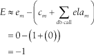
The following Oracle8i trace file excerpt shows the effect of quantization error:
WAIT #103: nam='db file sequential read' ela= 0 p1=1 p2=3051 p3=1
WAIT #103: nam='db file sequential read' ela= 0 p1=1 p2=6517 p3=1
WAIT #103: nam='db file sequential read' ela= 0 p1=1 p2=5347 p3=1
FETCH #103:c=0,e=1,p=3,cr=15,cu=0,mis=0,r=1,dep=2,og=4,tim=116694745
This fetch call motivated exactly three wait events. We know
that the c, e, and ela times shown here should be related by
the approximation:
On a low-load system, the amount by which the two sides of
this approximation are unequal is an indication of the total
quantization error present in the five measurements (one c value, one e value, and three ela values):

Given that individual gettimeofday calls account for only a few
microseconds of measurement intrusion error on most systems,
quantization error is the prominent factor contributing to the
1-centisecond (cs) “gap” in the trace data.
The following Oracle8i trace file excerpt shows the simplest possible over-counting of elapsed time, resulting in a negative amount of unaccounted-for time:
WAIT #96: nam='db file sequential read' ela= 0 p1=1 p2=1691 p3=1
FETCH #96:c=1,e=0,p=1,cr=4,cu=0,mis=0,r=1,dep=1,og=4,tim=116694789
Here, we have E = -1 cs:
In this case of a “negative gap” like the one shown here, we
cannot appeal to the effects of measurement intrusion for
explanation; the measurement intrusion effect can create only
positive unaccounted-for time. It might have
been possible that a CPU consumption double-count had taken place;
however, this isn’t the case here, because the value ela= 0 means that no CPU time was counted
in the wait event at all. In this case, quantization error has had a
dominating influence, resulting in the over-attribution of time
within the fetch.
Although Oracle9i uses improved output resolution in its timing statistics, Oracle9i is by no means immune to the effects of quantization error, as shown in the following trace file excerpt with E > 0:
WAIT #5: nam='db file sequential read' ela= 11597 p1=1 p2=42463 p3=1
FETCH #5:c=0,e=12237,p=1,cr=3,cu=0,mis=0,r=1,dep=2,og=4,tim=1023745094799915
In this example, we have E = 640 μs:
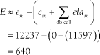
Some of this error is certainly quantization error (it’s impossible that the total CPU consumption of this fetch was actually zero). A few microseconds are the result of measurement intrusion error.
Finally, here is an example of an E < 0 quantization error in Oracle9i trace data:
WAIT #34: nam='db file sequential read' ela= 16493 p1=1 p2=33254 p3=1
WAIT #34: nam='db file sequential read' ela= 11889 p1=2 p2=89061 p3=1
FETCH #34:c=10000,e=29598,p=2,cr=5,cu=0,mis=0,r=1,dep=3,og=4,tim=1017039276445157
In this case, we have E = -8784 μs:

It is possible that some CPU consumption double-counting has occurred in this case. It is also likely that the effect of quantization error is a dominant contributor to the attribution of time to the fetch call. The 8,784-μs over-attribution is evidence that the actual total CPU consumption of the database call was probably only about (10,000 - 8,784) μs = 1,216 μs.
Bounds of Quantization Error
The amount of quantization error present in Oracle’s
timing statistics cannot be measured directly. However, the
statistical properties of quantization error can be analyzed in
extended SQL trace data. First, there’s a limit
to how much quantization error there can be in a given set of trace
data. It is easy to imagine the maximum quantization error that a
set of elapsed durations like Oracle’s e and ela statistics might contribute. The worst
total quantization error for a sequence of e and ela statistics occurs when all the
individual quantization errors are at their maximum magnitude
and the signs of the quantization errors all
line up.
Figure 7-9 exhibits the type of behavior that I’m describing. This drawing depicts eight very-short-duration system calls that happen to all cross an interval timer’s clock ticks. The actual duration of each event is practically zero, but the measured duration of each event is one clock tick. The total actual duration of the system calls shown is practically zero, but the total measured duration is 8 clock ticks. For this set of n = 8 system calls, the total quantization error is essentially nr x , where r x is, as described previously, the resolution of the interval timer upon which the x characteristic is measured.

It shouldn’t take you long to notice that the situation in Figure 7-9 is horribly contrived to suit my purpose of illustrating a point. For things to work out this way in reality is extremely unlikely. The probability that n quantization errors will all have the same sign is only 0.5 n . The probability of having n = 8 consecutive negative quantization errors is only 0.00390625 (that’s only about four chances in a thousand). There’s less than one chance in 1080 that n = 266 statistics will all have quantization errors with the same sign.
For long lists of elapsed duration statistics, it is virtually impossible for all the quantization errors to “point in the same direction.” Yet, my contrivance in Figure 7-9 goes even further. It assumes that the magnitude of each quantization error is maximized. The odds of this happening are even more staggeringly slim than for the signs to line up. For example, the probability that the magnitude of each of n given quantization error values exceeds 0.9 is only (1 - 0.9) n . The odds of having each of n = 266 quantization error magnitudes exceed 0.9 are one in 10266.
For n quantization errors to all have the same sign and all have magnitudes greater than m, the probability is the astronomically unlikely product of both probabilities I’ve described:
| P(n quantization error values areall greater than m or all less than -m)= (0.5) n (1 - m) n |
Quantization errors for elapsed durations (like Oracle
e and ela statistics) are random numbers in the
range:
| -r x < E < r x |
where r
x is the resolution of the
interval timer from which the x
statistic (where x is either
e or ela) is obtained.
Because negative and positive quantization errors occur with
equal probability, the average quantization error for a given set of
statistics tends toward zero, even for large trace files. Using the
central limit theorem developed by Pierre Simon
de Laplace in 1810, you can even predict the probability that
quantization errors for Oracle e
and ela statistics will exceed a
specified threshold for a trace file containing a given number of
statistics.
I’ve begun work to compute the probability that a trace file’s
total quantization error (including the error
contributed by c statistics) will
exceed a given threshold; however, I have not yet completed that
research. The problem in front of me is to calculate the
distribution of the quantization error produced by c, which, as I’ve said already, is
complicated by the nature of how c is tallied by polling. I intend to
document my research in this area in a future project.
Happily, there are several pieces of good news about quantization error that make not yet knowing how to quantify it quite bearable:
In the many hundreds of Oracle trace files that we have analyzed at http://www.hotsos.com, it has been extremely uncommon for a properly collected (see Chapter 6) file’s total unaccounted-for duration to exceed about 10% of total response time.
In spite of the possibilities afforded by both quantization error and CPU consumption double-counting, it is apparently extremely rare for a trace file to contain negative unaccounted-for time whose magnitude exceeds about 10% of total response time.
In cases where unaccounted-for time accounts for more than 25% of a properly collected trace file’s response time, the unaccounted-for time is almost always caused by one of the two remaining phenomena that I’ll discuss in the following sections.
The presence of quantization error has not yet hindered our ability to properly diagnose the root causes of performance problems by analyzing only Oracle extended SQL trace data, even in Oracle8i trace files in which all statistics are reported with only one-centisecond resolution.
Quantization error becomes even more of a non-issue in Oracle9i with the improvement in statistical resolution.
Sometimes, the effect of quantization error can cause loss of faith in the validity of Oracle’s trace data. Perhaps nothing can be more damaging to your morale in the face of a tough problem than to gather the suspicion that the data you’re counting on might be lying to you. A firm understanding of the effects of quantization error is possibly your most important tool in keeping your faith.
Time Spent Not Executing
To understand a fourth cause of unaccounted-for time in a properly collected Oracle trace file, let’s perform a brief thought experiment. Imagine a program P that consumes exactly ten seconds of user-mode CPU time and produces an output on your terminal. Imagine that you were to run this program in a loop on a system with one CPU. If you were the only user connected to this system, you should expect response time of ten seconds for each execution of P.
If you were to observe the CPU utilization of this single-CPU system during your single-user repetitive execution of P, you would probably notice your CPU running at 100% utilization for the duration of your job. But what if you were to add a second instance of the P loop on the single-CPU system? In any ten-second elapsed time interval, there is only ten seconds’ worth of CPU capacity available on the single-CPU machine. We thus cannot expect to accomplish two complete executions of a program that consumes ten seconds of capacity in one ten-second interval. We would expect that the response time of each P would increase to roughly 20 seconds each. That’s how long it would take for one CPU to provide ten seconds’ worth of CPU capacity to each of two competing processes, if its capacity were to be dispensed fairly and in small time slices to the two competing processes.
Instrumenting the Experiment
Let’s assume that we had instrumented our code in a manner similar to how the Oracle kernel does it, as I’ve shown in Example 7-6.
e0 = gettimeofday;
c0 = getrusage;
P;                        # remember, P makes no system calls
c1 = getrusage;
e1 = gettimeofday;
e = e1 - e0;
c = (c1.stime + c1.utime) - (c0.stime + c0.utime);
printf "e=%.0fs, c=%.0fs
", e, c;
Then we should expect approximately the timing output shown in Table 7-2 for each given concurrency level on a single-CPU system. You should expect our program P to consume the same amount of total CPU capacity, regardless of how busy the system is. But of course, since the CPU capacity of the system is being shared more and more thinly across users as we increase the concurrency level, you should expect for the program to execute for longer and longer elapsed times before being able to obtain the ten seconds of CPU time that it needs.
Number of users running P concurrently | Timing output |
1 | |
2 | |
3 | |
4 | |
The table shows what we expected to see, but notice that we now have created a “problem with missing time” in some of our measurements. Remember our performance model: the elapsed time of a program is supposed to approximately equal the time spent consuming CPU capacity plus the time spent executing instrumented “wait events,” as in:
However, even in the two-user case, this works out to:
| 20 ≈ 10 + 0 |
We can use the substitution ela = 0 because we know our program
executes no instrumented “wait events” whatsoever. All our program
does is consume some CPU capacity and then print the result. (And
even the printf statement can be
eliminated as a suspect because the call to it occurs
outside of the domain of the timer calls.) As
you can plainly see, c +
Σ ela = 10 is a really lousy approximation
of e = 20. Where did the
“missing time” go? In our Table 7-2 cases, the
problem just keeps getting worse as user concurrency increases.
Where have we gone wrong in our instrumentation of P?
Process States and Transitions Revisited
The answer is easy to understand after looking again at Figure 7-1. Recall that even when a process is executing happily along in user running state, a system clock interrupt occurs on most systems every 1/100th of a second. This regularly scheduled interrupt transitions each running process into the kernel running state to service the interrupt. Once in kernel running state, the process saves its current context and then executes the scheduler subroutine (see Section 7.1.2 earlier in this chapter). If there is a process in the ready to run state, then the system’s scheduling policy may dictate that the running process must be preempted, and the ready to run process be scheduled and given an opportunity to consume CPU capacity itself.
When this happens, note what happens to our originally running process. When it is interrupted, it is transitioned immediately to kernel running state. Note in particular that the process does not get the chance to execute any application code to see what time it is when this happens. When the process is preempted, it is transitioned to ready to run state, where it waits until it is scheduled. When it is finally scheduled (perhaps only a mere 10 milliseconds later), it spends enough time in kernel running state to reinstate its context, and then it returns to user running state, right where it left off.
How did the preemption activity affect the timing data for the
process? The CPU time spent in kernel running state while the
scheduler was preparing for the process’s preemption counts as CPU
time consumed by the process. But time spent in ready to run state
did not count as CPU time consumed by the
process. However, when the process had completed its work on
P, the difference e=e1-e0 of course included
all time spent in all
states of the process state transition diagram. The net effect is
that all the time spent in ready to run state continues to tally on
the e clock, but it’s not
accounted for as CPU capacity consumption, or for anything else that
the application is aware of for that matter. It’s as if the process
had been conked on the head and then awoken, with no way to account
for what happened to the time spent out of consciousness.
This is what happens to each process as more concurrent processes were added to the mix shown in Table 7-2. Of course, the more processes there were waiting in ready to run state, the more each process had to wait for its turn at the CPU. The longer the wait, the longer the program’s elapsed time. For three and four users, the unaccounted-for time increases proportionally. It’s simply a problem of a constant-sized pie (CPU capacity) being divvied up among more and more pie-eaters (users running P). There’s really nothing in need of “repair” about the instrumentation upon P. What you need is to understand how to estimate how much of the unaccounted-for time is likely to be due to time spent not executing.
The existence and exact size of this gap is of immense value to the Oracle performance analyst. The size of this gap permits you to use extended SQL trace data to identify when performance problems are caused by excessive swapping or time spent in the CPU run queue.
Un-Instrumented Oracle Kernel Code
The final cause of missing time in a trace file that
I’ll cover is the category consisting of un-instrumented
Oracle kernel code. As you’ve now seen, Oracle provides
instrumentation for database calls in the form of c and e
data, which represent total CPU consumption and total elapsed
duration, respectively. For segments of Oracle kernel code that can
consume significant response time but not much CPU capacity, Oracle
Corporation gives us the “wait event” instrumentation, complete with
an elapsed time and a distinguishing name for the code segment being
executed.
Chapter 11 lists the
number of code segments that are instrumented in a few popular
releases of the Oracle kernel since 7.3.4. Notice that the number
grows significantly with each release listed in the table. There are,
for example, 146 more instrumented system calls in release 9.2.0 than
there are in release 8.1.7. Certainly, some of these newly
instrumented events represent new product features. It is possible
that some new names in V$EVENT_NAME
correspond to code segments that were present but just not yet
instrumented in an earlier Oracle kernel release.
Effect
When Oracle Corporation leaves a sequence of kernel instructions un-instrumented, the missing time becomes apparent in one of two ways:
- Missing time within a database call
Any un-instrumented code that occurs within the context of a database call will leave a gap between the database call’s elapsed duration (e) and the value of c + Σ ela for the call. Within the trace file, the phenomenon will be indistinguishable from the time spent not executing problem that I described earlier. On systems that do not exhibit much paging or swapping, the presence of a large gap (Δ) in the following equation for an entire trace file is an indicator of an un-instrumented time problem:
To envision this problem, imagine what would happen if a five-second database file read executed by a fetch were un-instrumented. The elapsed time for the fetch (
e) would include the five-second duration, but neither the total CPU consumption for the fetch (c) nor the wait event durations (elavalues) would be large enough to account for the whole elapsed duration.- Missing time between database calls
Any un-instrumented code that occurs outside of the context of a database call cannot be detected in the same manner as un-instrumented code that occurs within a database call. You can detect missing time between calls in one of two ways. First, a sequence of between-call events with no intervening database calls is an indication of un-instrumented Oracle kernel code path. Second, you can detect un-instrumented calls by inspecting
timstatistic values within a trace file. If you see “adjacent”timvalues that are much farther apart in time than the intervening database call and wait event lines can account for, then you’ve discovered this problem. A trace file exhibits this issue if it has a large Δ value in the formula in which R denotes the known response time for which the trace file was supposed to account:Oracle bug number 2425312 is one example of this problem. It is a case in which entire database calls executed through the PL/SQL remote procedure call (RPC) interface emit no trace data whatsoever. The result is a potentially enormous gap in the time accounting within a trace file.

In practice you may never encounter a situation in which un-instrumented system calls will consume an important proportion of a program’s elapsed time. We encounter the phenomenon at a rate of fewer than five per thousand trace files at http://www.hotsos.com. One case of un-instrumented database activity is documented as bug number 2425312 at Oracle MetaLink. You may encounter this bug if you trace Oracle Forms applications with embedded (client-side) PL/SQL. You will perhaps encounter other cases in which un-instrumented time materially affects your analysis, but those cases will be rare.
Trace Writing
You will encounter at least one un-instrumented system call
every time you use SQL trace, although its performance impact is
usually small. It is the write
call that the Oracle kernel uses to write SQL trace output to the
trace file. Using strace allows
you to see quite plainly how the Oracle kernel writes each line of
data to a trace file. Of the several hundred extended SQL trace
files collected at http://www.hotsos.com by
the time of this writing, fewer than 1% exhibit accumulation of
unaccounted-for time that might be explained by slow trace file
writing. However, you should follow these recommendations to reduce
the risk that the very act of tracing an application program will
materially degrade the performance of an application:
Check with Oracle MetaLink to ensure that your system is not susceptible to Oracle kernel bugs that might unnecessarily impede the performance of trace file writing. For example, bug number 2202613 affects the performance of trace file writing on some Microsoft Windows 2000 ports. Bug number 1210242 needlessly degrades Oracle performance while tracing is activated.
Place your
USER_DUMP_DESTandBACKGROUND_DUMP_DESTdirectories on efficient I/O channels. Don’t write trace data to your root filesystem or the oldest, slowest disk drive on your system. Although the outcome of the diagnostic process will often be significant performance improvement, no analyst wants to be accused of even temporarily degrading the performance of an application.Keep load that competes with trace file I/O as low as possible during a trace. For example, avoid tracing more than one session at a time to the same I/O device. Exceptions include application programs that naturally emit more than one trace file, such as parallel operations or any program that distributes workload over more than one Oracle server processes.
Don’t let the overhead of writing to trace files deter you from using extended SQL trace data as a performance diagnostic tool. Keep the overhead in perspective. The potential overhead is not noticeable in most cases. Even if the performance overhead were nearly unbearable, the overhead of tracing a program once is a worthwhile investment if the diagnosis results in either of the following outcomes:
Exercises
Install a system call trace utility like
straceon your system. Use it to trace an Oracle kernel process. In a separate window, view the SQL trace output as it is emitted (usingtail -for a similar command). What timing calls does the Oracle kernel make on your system? In what sequence are the timing calls made? Does your system’s behavior resemble the behavior described in Example 7-2?Run the program listed in Example 7-4 on your system. What is the average measurement intrusion effect of one
gettimeofdaycall on your system?The Perl program in Example 7-7 saves the values returned from a rapid-fire sequence of
timessystem calls. It traverses the list of saved values and prints a value only if it differs from the prior value in the list. What, if anything, does running this program indicate about the resolution of CPU resource accounting on your system?Example 7-7. A Perl program that executes a rapid-fire sequence of times system calls#!/usr/bin/perl use strict; use warnings; use IO::File; autoflush STDOUT 1; my @times = (times)[0]; while ((my $t = (times)[0]) - $times[0] < 1) { push @times, $t; } print scalar @times, " distinct times "; my $prior = ''; for my $time (@times) { print "$time " if $time ne $prior; $prior = $time; }At http://www.hotsos.com, we have several millions of lines of Oracle8i trace data that resemble the following:
FETCH #1:c=1,e=0,p=0,cr=0,cu=0,mis=0,r=10,dep=0,og=3,tim=17132884
Explain how this can occur.
In Oracle9i, trace file lines like the following occur as frequently as the phenomenon described in the previous exercise:
PARSE #7:c=10000,e=2167,p=0,cr=0,cu=0,mis=1,r=0,dep=1,og=0,tim=1016096093915846
Explain how this can occur. How different is this phenomenon from the one described in the previous exercise?
Write a program to test the thought experiment shown in Example 7-6. Explain any major differences between its output and the output of the thought experiment shown in Table 7-2.
Trace client programs that use different Oracle interfaces on your system, such as:
PL/SQL RPC calls issued by client-side PL/SQL within Oracle Forms applications
Java RMI calls between the client VM and server VM
Do they result in unexpectedly large amounts of unaccounted-for time?