
by Richard S. Wright, Jr.
WHAT YOU'LL LEARN IN THIS CHAPTER:
How To | Functions You'll Use |
|---|---|
Establish your position in the scene |
|
Position objects within the scene |
|
Scale objects |
|
Establish a perspective transformation |
|
Perform your own matrix transformations |
|
|
|
In Chapter 3, “Drawing in Space: Geometric Primitives and Buffers,” you learned how to draw points, lines, and various primitives in 3D. To turn a collection of shapes into a coherent scene, you must arrange them in relation to one another and to the viewer. In this chapter, you start moving shapes and objects around in your coordinate system. (Actually, you don't move the objects, but rather shift the coordinate system to create the view you want.) The ability to place and orient your objects in a scene is a crucial tool for any 3D graphics programmer. As you will see, it is actually convenient to describe your objects' dimensions around the origin and then transform the objects into the desired position.
In most books on 3D graphics programming, yes, this would be the dreaded math chapter. However, you can relax; we take a more moderate approach to these principles than some texts.
The keys to object and coordinate transformations are two matrices maintained by OpenGL. To familiarize you with these matrices, this chapter strikes a compromise between two extremes in computer graphics philosophy. On one hand, we could warn you, “Please review a textbook on linear algebra before reading this chapter.” On the other hand, we could perpetuate the deceptive reassurance that you can “learn to do 3D graphics without all those complex mathematical formulas.” But we don't agree with either camp.
In reality, you can get along just fine without understanding the finer mathematics of 3D graphics, just as you can drive your car every day without having to know anything at all about automotive mechanics and the internal combustion engine. But you had better know enough about your car to realize that you need an oil change every so often, that you have to fill the tank with gas regularly, and that you must change the tires when they get bald. This knowledge makes you a responsible (and safe!) automobile owner. If you want to be a responsible and capable OpenGL programmer, the same standards apply. You need to understand at least the basics so you know what can be done and what tools best suit the job. If you are a beginner, you will find that, with some practice, matrix math and vectors will gradually make more and more sense, and you will develop a more intuitive (and powerful) ability to make full use of the concepts we introduce in this chapter.
So, even if you don't already have the ability to multiply two matrices in your head, you need to know what matrices are and that they are the means to OpenGL's 3D magic. But before you go dusting off that old linear algebra textbook (doesn't everyone have one?), have no fear: OpenGL does all the math for you. Think of using OpenGL as using a calculator to do long division when you don't know how to do it on paper. Although you don't have to do it yourself, you still know what it is and how to apply it. See—you can eat your cake and have it, too!
If you think about it, most 3D graphics aren't really 3D. We use 3D concepts and terminology to describe what something looks like; then this 3D data is “squished” onto a 2D computer screen. We call the process of squishing 3D data down into 2D data projection, and we introduced both orthographic and perspective projections back in Chapter 1, “Introduction to 3D Graphics and OpenGL.” We refer to the projection whenever we want to describe the type of transformation (orthographic or perspective) that occurs during projection, but projection is only one of the different types of transformations that occurs in OpenGL. Transformations also allow you to rotate objects around; move them about; and even stretch, shrink, and warp them.
Three types of geometric transformations occur between the time you specify your vertices and the time they appear on the screen: viewing, modeling, and projection. In this section, we examine the principles of each type of transformation, which are summarized in Table 4.1.
An important concept throughout this chapter is that of eye coordinates. Eye coordinates are from the viewpoint of the observer, regardless of any transformations that may occur; you can think of them as “absolute” screen coordinates. Thus, eye coordinates are not real coordinates; instead, they represent a virtual fixed coordinate system that is used as a common frame of reference. All the transformations discussed in this chapter are described in terms of their effects relative to the eye coordinate system.
Figure 4.1 shows the eye coordinate system from two viewpoints. On the left (a), the eye coordinates are represented as seen by the observer of the scene (that is, perpendicular to the monitor). On the right (b), the eye coordinate system is rotated slightly so you can better see the relation of the z-axis. Positive x and y are pointed right and up, respectively, from the viewer's perspective. Positive z travels away from the origin toward the user, and negative z values travel farther away from the viewpoint into the screen.

When you draw in 3D with OpenGL, you use the Cartesian coordinate system. In the absence of any transformations, the system in use is identical to the eye coordinate system just described.
The viewing transformation is the first to be applied to your scene. It is used to determine the vantage point of the scene. By default, the point of observation in a perspective projection is at the origin (0,0,0) looking down the negative z-axis (“into” the monitor screen). This point of observation is moved relative to the eye coordinate system to provide a specific vantage point. When the point of observation is located at the origin, objects drawn with positive z values are behind the observer.
The viewing transformation allows you to place the point of observation anywhere you want and look in any direction. Determining the viewing transformation is like placing and pointing a camera at the scene.
In the grand scheme of things, you must specify the viewing transformation before any other transformations. The reason is that it appears to move the current working coordinate system in respect to the eye coordinate system. All subsequent transformations then occur based on the newly modified coordinate system. Later, you'll see more easily how this works, when we actually start looking at how to make these transformations.
Modeling transformations are used to manipulate your model and the particular objects within it. These transformations move objects into place, rotate them, and scale them. Figure 4.2 illustrates three of the most common modeling transformations that you will apply to your objects. Figure 4.2a shows translation, where an object is moved along a given axis. Figure 4.2b shows a rotation, where an object is rotated about one of the axes. Finally, Figure 4.2c shows the effects of scaling, where the dimensions of the object are increased or decreased by a specified amount. Scaling can occur nonuniformly (the various dimensions can be scaled by different amounts), so you can use scaling to stretch and shrink objects.

The final appearance of your scene or object can depend greatly on the order in which the modeling transformations are applied. This is particularly true of translation and rotation. Figure 4.3a shows the progression of a square rotated first about the z-axis and then translated down the newly transformed x-axis. In Figure 4.3b, the same square is first translated down the x-axis and then rotated around the z-axis. The difference in the final dispositions of the square occurs because each transformation is performed with respect to the last transformation performed. In Figure 4.3a, the square is rotated with respect to the origin first. In 4.3b, after the square is translated, the rotation is performed around the newly translated origin.
The viewing and modeling transformations are, in fact, the same in terms of their internal effects as well as their effects on the final appearance of the scene. The distinction between the two is made purely as a convenience for the programmer. There is no real difference between moving an object backward and moving the reference system forward; as shown in Figure 4.4, the net effect is the same. (You experience this effect firsthand when you're sitting in your car at an intersection and you see the car next to you roll forward; it might seem to you that your own car is rolling backward.) The term modelview indicates that you can think of this transformation either as the modeling transformation or the viewing transformation, but in fact there is no distinction; thus, it is the modelview transformation.

The viewing transformation, therefore, is essentially nothing but a modeling transformation that you apply to a virtual object (the viewer) before drawing objects. As you will soon see, new transformations are repeatedly specified as you place more objects in the scene. By convention, the initial transformation provides a reference from which all other transformations are based.
The projection transformation is applied to your vertices after the modelview transformation. This projection actually defines the viewing volume and establishes clipping planes. The clipping planes are plane equations in 3D space that OpenGL uses to determine whether geometry can be seen by the viewer.. More specifically, the projection transformation specifies how a finished scene (after all the modeling is done) is projected to the final image on the screen. You learn about two types of projections in this chapter: orthographic and perspective.
In an orthographic, or parallel, projection, all the polygons are drawn onscreen with exactly the relative dimensions specified. Lines and polygons are mapped directly to the 2D screen using parallel lines, which means no matter how far away something is, it is still drawn the same size, just flattened against the screen. This type of projection is typically used for CAD or for rendering two-dimensional images such as blueprints or two-dimensional graphics such as text or onscreen menus.
A perspective projection shows scenes more as they appear in real life instead of as a blueprint. The trademark of perspective projections is foreshortening, which makes distant objects appear smaller than nearby objects of the same size. Lines in 3D space that might be parallel do not always appear parallel to the viewer. With a railroad track, for instance, the rails are parallel, but using perspective projection, they appear to converge at some distant point.
The benefit of perspective projection is that you don't have to figure out where lines converge or how much smaller distant objects are. All you need to do is specify the scene using the modelview transformations and then apply the perspective projection. OpenGL works all the magic for you. Figure 4.5 compares orthographic and perspective projections on two different scenes.

Orthographic projections are used most often for 2D drawing purposes where you want an exact correspondence between pixels and drawing units. You might use them for a schematic layout, text, or perhaps a 2D graphing application. You also can use an orthographic projection for 3D renderings when the depth of the rendering has a very small depth in comparison to the distance from the viewpoint. Perspective projections are used for rendering scenes that contain wide open spaces or objects that need to have the foreshortening applied. For the most part, perspective projections are typical for 3D graphics. In fact, looking at a 3D object with an orthographic projection can be somewhat unsettling.
When all is said and done, you end up with a two-dimensional projection of your scene that will be mapped to a window somewhere on your screen. This mapping to physical window coordinates is the last transformation that is done, and it is called the viewport transformation. Usually, a one-to-one correspondence exists between the color buffer and window pixels, but this is not always strictly the case. In some circumstances, the viewport transformation remaps what are called “normalized” device coordinates to window coordinates. Fortunately, this is something you don't need to worry about.
Now that you're armed with some basic vocabulary and definitions of transformations, you're ready for some simple matrix mathematics. Let's examine how OpenGL performs these transformations and get to know the functions you call to achieve the desired effects.
The mathematics behind these transformations are greatly simplified by the mathematical notation of the matrix. You can achieve each of the transformations we have discussed by multiplying a matrix that contains the vertices (usually, this is a simple vector) by a matrix that describes the transformation. Thus, all the transformations achievable with OpenGL can be described as the product of two or more matrix multiplications.
The Matrix is not only a wildly popular Hollywood movie trilogy, but an exceptionally powerful mathematical tool that greatly simplifies the process of solving one or more equations with variables that have complex relationships to one another. One common example of this, near and dear to the hearts of graphics programmers, is coordinate transformations. For example, if you have a point in space represented by x, y, and z coordinates, and you need to know where that point is if you rotate it some number of degrees around some arbitrary point and orientation, you would use a matrix. Why? Because the new x coordinate depends not only on the old x coordinate and the other rotation parameters, but also on what the y and z coordinates were as well. This kind of dependency between the variables and solution is just the sort of problem that matrices excel at. For fans of the Matrix movies who have a mathematical inclination, the term matrix is indeed an appropriate title.
Mathematically, a matrix is nothing more than a set of numbers arranged in uniform rows and columns—in programming terms, a two-dimensional array. A matrix doesn't have to be square, but each row or column must have the same number of elements as every other row or column in the matrix. Figure 4.6 presents some examples of matrices. They don't represent anything in particular, but serve only to demonstrate matrix structure. Note that it is also valid for a matrix to have a single column or row. A single row or column of numbers is also more simply called a vector, and vectors also have some interesting and useful applications all their own.

Matrix and vector are two important terms that you will see often in 3D graphics programming literature. When dealing with these quantities, you will also see the term scalar. A scalar is just an ordinary single number used to represent magnitude or a specific quantity (you know—a regular old plain simple number…like before you cared or had all this jargon added to your vocabulary).
Matrices can be multiplied and added together, but they can also be multiplied by vectors and scalar values. Multiplying a point (a vector) by a matrix (a transformation) yields a new transformed point (a vector). Matrix transformations are actually not too difficult to understand but can be intimidating at first. Because an understanding of matrix transformations is fundamental to many 3D tasks, you should still make an attempt to become familiar with them. Fortunately, only a little understanding is enough to get you going and doing some pretty incredible things with OpenGL. Over time, and with a little more practice and study (see Appendix A, “Further Reading”), you will master this mathematical tool yourself. In the meantime, you can find a number of useful matrix and vector functions and features available, with source code, in the glTools library (see the common directory under the samples directory) on the CD that accompanies this book.
To effect the types of transformations described in this chapter, you modify two matrices in particular: the modelview matrix and projection matrix. Don't worry; OpenGL provides some high-level functions that you can call for these transformations. After you've mastered the basics of the OpenGL API, you will undoubtedly start trying some of the more advanced 3D rendering techniques. Only then will you need to call the lower-level functions that actually set the values contained in the matrices.
The road from raw vertex data to screen coordinates is a long one. Figure 4.7 provides a flowchart of this process. First, your vertex is converted to a 1×4 matrix in which the first three values are the x, y, and z coordinates. The fourth number is a scaling factor that you can apply manually by using the vertex functions that take four values. This is the w coordinate, usually 1.0 by default. You will seldom modify this value directly.

The vertex is then multiplied by the modelview matrix, which yields the transformed eye coordinates. The eye coordinates are then multiplied by the projection matrix to yield clip coordinates. This effectively eliminates all data outside the viewing volume. The clip coordinates are then divided by the w coordinate to yield normalized device coordinates. The w value may have been modified by the projection matrix or the modelview matrix, depending on the transformations that occurred. Again, OpenGL and the high-level matrix functions hide this process from you.
Finally, your coordinate triplet is mapped to a 2D plane by the viewport transformation.
The modelview matrix is a 4×4 matrix that represents the transformed coordinate system you are using to place and orient your objects. The vertices you provide for your primitives are used as a single-column matrix and multiplied by the modelview matrix to yield new transformed coordinates in relation to the eye coordinate system.
In Figure 4.8, a matrix containing data for a single vertex is multiplied by the modelview matrix to yield new eye coordinates. The vertex data is actually four elements with an extra value, w, that represents a scaling factor. This value is set by default to 1.0, and rarely will you change it yourself.

Let's consider an example that modifies the modelview matrix. Say you want to draw a cube using the GLUT library's glutWireCube function. You simply call
glutWireCube(10.0f);
A cube that measures 10 units on a side is then centered at the origin. To move the cube up the y-axis by 10 units before drawing it, you multiply the modelview matrix by a matrix that describes a translation of 10 units up the y-axis and then do your drawing. In skeleton form, the code looks like this:
// Construct a translation matrix for positive 10 Y
...

// Multiply it by the modelview matrix
...

// Draw the cube
glutWireCube(10.0f);
Actually, such a matrix is fairly easy to construct, but it requires quite a few lines of code. Fortunately, OpenGL provides a high-level function that performs this task for you:
void glTranslatef(GLfloat x, GLfloat y, GLfloat z);
This function takes as parameters the amount to translate along the x, y, and z directions. It then constructs an appropriate matrix and does the multiplication. The pseudocode looks like the following, and the effect is illustrated in Figure 4.9:
// Translate up the y-axis 10 units
glTranslatef(0.0f, 10.0f, 0.0f);

// Draw the cube
glutWireCube(10.0f);
To rotate an object about one of the three coordinate axes, or indeed any arbitrary vector, you have to devise a rotation matrix. Again, a high-level function comes to the rescue:
glRotatef(GLfloat angle, GLfloat x, GLfloat y, GLfloat z);
Here, we perform a rotation around the vector specified by the x, y, and z arguments. The angle of rotation is in the counterclockwise direction measured in degrees and specified by the argument angle. In the simplest of cases, the rotation is around only one of the axes.
You can also perform a rotation around an arbitrary axis by specifying x, y, and z values for that vector. To see the axis of rotation, you can just draw a line from the origin to the point represented by (x,y,z). The following code rotates the cube by 45° around an arbitrary axis specified by (1,1,1), as illustrated in Figure 4.10:

A scaling transformation increases the size of your object by expanding all the vertices along the three axes by the factors specified. The function
glScalef(GLfloat x, GLfloat y, GLfloat z);
multiplies the x, y, and z values by the scaling factors specified.
Scaling does not have to be uniform, and you can use it to both stretch or squeeze objects along different directions. For example, the following code produces a cube that is twice as large along the x- and z-axes as the cubes discussed in the previous examples, but still the same along the y-axis. The result is shown in Figure 4.11.
// Perform the scaling transformation
glScalef(2.0f, 1.0f, 2.0f);

// Draw the cube
glutWireCube(10.0f);
About now, you might be wondering why we had to bother with all this matrix stuff in the first place. Can't we just call these transformation functions to move our objects around and be done with it? Do we really need to know that it is the modelview matrix that is modified?
The answer is yes and no (but it's no only if you are drawing a single object in your scene). The reason is that the effects of these functions are cumulative. Each time you call one, the appropriate matrix is constructed and multiplied by the current modelview matrix. The new matrix then becomes the current modelview matrix, which is then multiplied by the next transformation, and so on.
Suppose you want to draw two spheres—one 10 units up the positive y-axis and one 10 units out the positive x-axis, as shown in Figure 4.12. You might be tempted to write code that looks something like this:
// Go 10 units up the y-axis
glTranslatef(0.0f, 10.0f, 0.0f);

// Draw the first sphere
glutSolidSphere(1.0f,15,15);

// Go 10 units out the x-axis
glTranslatef(10.0f, 0.0f, 0.0f);

// Draw the second sphere
glutSolidSphere(1.0f);

Consider, however, that each call to glTranslate is cumulative on the modelview matrix, so the second call translates 10 units in the positive x direction from the previous translation in the y direction. This yields the results shown in Figure 4.13.

You can make an extra call to glTranslate to back down the y-axis 10 units in the negative direction, but this makes some complex scenes difficult to code and debug—not to mention that you throw extra transformation math at the CPU. A simpler method is to reset the modelview matrix to a known state—in this case, centered at the origin of the eye coordinate system.
You reset the origin by loading the modelview matrix with the identity matrix. The identity matrix specifies that no transformation is to occur, in effect saying that all the coordinates you specify when drawing are in eye coordinates. An identity matrix contains all 0s, with the exception of a diagonal row of 1s. When this matrix is multiplied by any vertex matrix, the result is that the vertex matrix is unchanged. Figure 4.14 shows this equation. Later in the chapter, we discuss in more detail why these numbers are where they are.

As we've already stated, the details of performing matrix multiplication are outside the scope of this book. For now, just remember this: Loading the identity matrix means that no transformations are performed on the vertices. In essence, you are resetting the modelview matrix back to the origin.
The following two lines load the identity matrix into the modelview matrix:
glMatrixMode(GL_MODELVIEW);
glLoadIdentity();
The first line specifies that the current operating matrix is the modelview matrix. After you set the current operating matrix (the matrix that your matrix functions are affecting), it remains the active matrix until you change it. The second line loads the current matrix (in this case, the modelview matrix) with the identity matrix.
Now, the following code produces results as shown earlier in Figure 4.12:
// Set current matrix to modelview and reset
glMatrixMode(GL_MODELVIEW);
glLoadIdentity();

// Go 10 units up the y-axis
glTranslatef(0.0f, 10.0f, 0.0f);

// Draw the first sphere
glutSolidSphere(1.0f, 15, 15);

// Reset modelview matrix again
glLoadIdentity();

// Go 10 units out the x-axis
glTranslatef(10.0f, 0.0f, 0.0f);

// Draw the second sphere
glutSolidSphere(1.0f, 15, 15);
Resetting the modelview matrix to identity before placing every object is not always desirable. Often, you want to save the current transformation state and then restore it after some objects have been placed. This approach is most convenient when you have initially transformed the modelview matrix as your viewing transformation (and thus are no longer located at the origin).
To facilitate this procedure, OpenGL maintains a matrix stack for both the modelview and projection matrices. A matrix stack works just like an ordinary program stack. You can push the current matrix onto the stack to save it and then make your changes to the current matrix. Popping the matrix off the stack restores it. Figure 4.15 shows the stack principle in action.

The stack depth can reach a maximum value that you can retrieve with a call to either
glGet(GL_MAX_MODELVIEW_STACK_DEPTH);
or
glGet(GL_MAX_PROJECTION_STACK_DEPTH);
If you exceed the stack depth, you get a GL_STACK_OVERFLOW error; if you try to pop a matrix value off the stack when there is none, you generate a OW errorGL_STACK_UNDERFLOW error. The stack depth is implementation dependent. For the Microsoft software implementation, the values are 32 for the modelview and 2 for the projection stack.
Let's put to use what we have learned. In the next example, we build a crude, animated model of an atom. This atom has a single sphere at the center to represent the nucleus and three electrons in orbit about the atom. We use an orthographic projection, as we have previously in this book.
Our ATOM program uses the GLUT timer callback mechanism (discussed in Chapter 2, “Using OpenGL”) to redraw the scene about 10 times per second. Each time the RenderScene function is called, the angle of revolution about the nucleus is incremented. Also, each electron lies in a different plane. Listing 4.1 shows the RenderScene function for this example, and the output from the ATOM program is shown in Figure 4.16.
Example 4.1. RenderScene Function from ATOM Sample Program
// Called to draw scene
void RenderScene(void)
{
    // Angle of revolution around the nucleus
    static GLfloat fElect1 = 0.0f;

    // Clear the window with current clearing color
    glClear(GL_COLOR_BUFFER_BIT | GL_DEPTH_BUFFER_BIT);

    // Reset the modelview matrix
    glMatrixMode(GL_MODELVIEW);
    glLoadIdentity();


    // Translate the whole scene out and into view
    // This is the initial viewing transformation
    glTranslatef(0.0f, 0.0f, -100.0f);

    // Red Nucleus

    glColor3ub(255, 0, 0);
    glutSolidSphere(10.0f, 15, 15);

    // Yellow Electrons

    glColor3ub(255,255,0);

    // First Electron Orbit
    // Save viewing transformation
    glPushMatrix();

    // Rotate by angle of revolution
    glRotatef(fElect1, 0.0f, 1.0f, 0.0f);

    // Translate out from origin to orbit distance
    glTranslatef(90.0f, 0.0f, 0.0f);

    // Draw the electron
    glutSolidSphere(6.0f, 15, 15);

    // Restore the viewing transformation
    glPopMatrix();

    // Second Electron Orbit
    glPushMatrix();
    glRotatef(45.0f, 0.0f, 0.0f, 1.0f);
    glRotatef(fElect1, 0.0f, 1.0f, 0.0f);
    glTranslatef(-70.0f, 0.0f, 0.0f);
    glutSolidSphere(6.0f, 15, 15);
    glPopMatrix();


    // Third Electron Orbit
    glPushMatrix();
    glRotatef(360.0f, -45.0f, 0.0f, 0.0f, 1.0f);
    glRotatef(fElect1, 0.0f, 1.0f, 0.0f);
    glTranslatef(0.0f, 0.0f, 60.0f);
    glutSolidSphere(6.0f, 15, 15);
    glPopMatrix();


    // Increment the angle of revolution
    fElect1 += 10.0f;
    if(fElect1 > 360.0f)
        fElect1 = 0.0f;

    // Show the image
    glutSwapBuffers();
}

Let's examine the code for placing one of the electrons, a couple of lines at a time. The first line saves the current modelview matrix by pushing the current transformation on the stack:
// First Electron Orbit
// Save viewing transformation
glPushMatrix();
Now the coordinate system appears to be rotated around the y-axis by an angle, fElect1:
// Rotate by angle of revolution
glRotatef(fElect1, 0.0f, 1.0f, 0.0f);
The electron is drawn by translating down the newly rotated coordinate system:
// Translate out from origin to orbit distance
    glTranslatef(90.0f, 0.0f, 0.0f);
Then the electron is drawn (as a solid sphere), and we restore the modelview matrix by popping it off the matrix stack:
// Draw the electron
    glutSolidSphere(6.0f, 15, 15);

    // Restore the viewing transformation
    glPopMatrix();
The other electrons are placed similarly.
In our examples so far, we have used the modelview matrix to position our vantage point of the viewing volume and to place our objects therein. The projection matrix actually specifies the size and shape of our viewing volume.
Thus far in this book, we have created a simple parallel viewing volume using the function glOrtho, setting the near and far, left and right, and top and bottom clipping coordinates. When the projection matrix is loaded with the identity matrix, the diagonal line of 1s specifies that the clipping planes extend from the origin to +1 or –1 in all directions. The projection matrix by itself does no scaling or perspective adjustments unless you load a perspective projection matrix.
The next two sample programs, ORTHO and PERSPECT, are not covered in detail from the standpoint of their source code. These examples use lighting and shading that we haven't covered yet to help highlight the differences between an orthographic and a perspective projection. These interactive samples make it much easier for you to see firsthand how the projection can distort the appearance of an object. If possible, you should run these examples while reading the next two sections.
An orthographic projection, used for most of this book so far, is square on all sides. The logical width is equal at the front, back, top, bottom, left, and right sides. This produces a parallel projection, which is useful for drawings of specific objects that do not have any foreshortening when viewed from a distance. This is good for CAD, 2D graphics such as text, or architectural drawings for which you want to represent the exact dimensions and measurements onscreen.
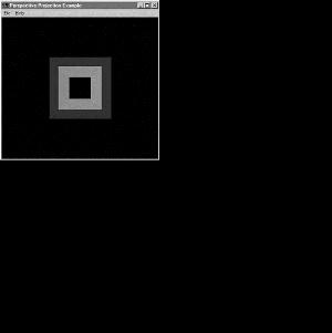
Figure 4.17 shows the output from the sample program ORTHO in this chapter's subdirectory on the CD. To produce this hollow, tube-like box, we used an orthographic projection just as we did for all our previous examples. Figure 4.18 shows the same box rotated more to the side so you can see how long it actually is.

In Figure 4.19, you're looking directly down the barrel of the tube. Because the tube does not converge in the distance, this is not an entirely accurate view of how such a tube appears in real life. To add some perspective, we must use a perspective projection.

A perspective projection performs perspective division to shorten and shrink objects that are farther away from the viewer. The width of the back of the viewing volume does not have the same measurements as the front of the viewing volume after being projected to the screen. Thus, an object of the same logical dimensions appears larger at the front of the viewing volume than if it were drawn at the back of the viewing volume.
The picture in our next example is of a geometric shape called a frustum. A frustum is a truncated section of a pyramid viewed from the narrow end to the broad end. Figure 4.20 shows the frustum, with the observer in place.

You can define a frustum with the function glFrustum. Its parameters are the coordinates and distances between the front and back clipping planes. However, glFrustum is not intuitive about setting up your projection to get the desired effects. The utility function gluPerspective is easier to use and somewhat more intuitive for most purposes:
void gluPerspective(GLdouble fovy, GLdouble aspect,
                     GLdouble zNear, GLdouble zFar);
Parameters for the gluPerspective function are a field-of-view angle in the vertical direction, the aspect ratio of the height to width, and the distances to the near and far clipping planes (see Figure 4.21). You find the aspect ratio by dividing the width (w) by the height (h) of the window or viewport.

Listing 4.2 shows how we change our orthographic projection from the previous examples to use a perspective projection. Foreshortening adds realism to our earlier orthographic projections of the square tube (see Figures 4.22, 4.23, and 4.24). The only substantial change we made for our typical projection code in Listing 4.2 was substituting the call to gluOrtho2D with gluPerspective.
Example 4.2. Setting Up the Perspective Projection for the PERSPECT Sample Program
// Change viewing volume and viewport.  Called when window is resized
void ChangeSize(GLsizei w, GLsizei h)
    {
    GLfloat fAspect;

    // Prevent a divide by zero
    if(h == 0)
        h = 1;

    // Set viewport to window dimensions
    glViewport(0, 0, w, h);

    fAspect = (GLfloat)w/(GLfloat)h;

    // Reset coordinate system
    glMatrixMode(GL_PROJECTION);
    glLoadIdentity();

    // Produce the perspective projection
    gluPerspective(60.0f, fAspect, 1.0, 400.0);

    glMatrixMode(GL_MODELVIEW);
    glLoadIdentity();
    }


We made the same changes to the ATOM example in ATOM2 to add perspective. Run the two side by side, and you see how the electrons appear to be smaller as they swing far away behind the nucleus.
For a more complete example showing modelview manipulation and perspective projections, we have modeled the Sun and the Earth/Moon system in revolution in the SOLAR example program. This is a classic example of nested transformations with objects being transformed relative to one another using the matrix stack. We have enabled some lighting and shading for drama so you can more easily see the effects of our operations. You'll learn about shading and lighting in the next two chapters.
In our model, the Earth moves around the Sun, and the Moon revolves around the Earth. A light source is placed at the center of the Sun, which is drawn without lighting to make it appear to be the glowing light source. This powerful example shows how easily you can produce sophisticated effects with OpenGL.
Listing 4.3 shows the code that sets up the projection and the rendering code that keeps the system in motion. A timer elsewhere in the program triggers a window redraw 10 times a second to keep the RenderScene function in action. Notice in Figures 4.25 and 4.26 that when the Earth appears larger, it's on the near side of the Sun; on the far side, it appears smaller.
Example 4.3. Code That Produces the Sun/Earth/Moon System
// Change viewing volume and viewport.  Called when window is resized
void ChangeSize(GLsizei w, GLsizei h)
    {
    GLfloat fAspect;

    // Prevent a divide by zero
    if(h == 0)
        h = 1;

    // Set viewport to window dimensions
    glViewport(0, 0, w, h);

    // Calculate aspect ratio of the window
    fAspect = (GLfloat)w/(GLfloat)h;

    // Set the perspective coordinate system
    glMatrixMode(GL_PROJECTION);
    glLoadIdentity();

    // Field of view of 45 degrees, near and far planes 1.0 and 425
    gluPerspective(45.0f, fAspect, 1.0, 425.0);

    // Modelview matrix reset
    glMatrixMode(GL_MODELVIEW);
    glLoadIdentity();
    }

// Called to draw scene
void RenderScene(void)
    {
    // Earth and Moon angle of revolution
    static float fMoonRot = 0.0f;
    static float fEarthRot = 0.0f;

    // Clear the window with current clearing color
    glClear(GL_COLOR_BUFFER_BIT | GL_DEPTH_BUFFER_BIT);

    // Save the matrix state and do the rotations
    glMatrixMode(GL_MODELVIEW);
    glPushMatrix();

    // Translate the whole scene out and into view
    glTranslatef(0.0f, 0.0f, -300.0f);

    // Set material color, to yellow
    // Sun
    glColor3ub(255, 255, 0);
    glDisable(GL_LIGHTING);
    glutSolidSphere(15.0f, 15, 15);
    glEnable(GL_LIGHTING);

    // Position the light after we draw the sun!
    glLightfv(GL_LIGHT0,GL_POSITION,lightPos);

    // Rotate coordinate system
    glRotatef(fEarthRot, 0.0f, 1.0f, 0.0f);

    // Draw the Earth
    glColor3ub(0,0,255);
    glTranslatef(105.0f,0.0f,0.0f);
    glutSolidSphere(15.0f, 15, 15);


    // Rotate from Earth-based coordinates and draw Moon
    glColor3ub(200,200,200);
    glRotatef(fMoonRot,0.0f, 1.0f, 0.0f);
    glTranslatef(30.0f, 0.0f, 0.0f);
    fMoonRot+= 15.0f;
    if(fMoonRot > 360.0f)
        fMoonRot = 0.0f;

    glutSolidSphere(6.0f, 15, 15);


    // Restore the matrix state
    glPopMatrix();    // Modelview matrix


    // Step earth orbit 5 degrees
    fEarthRot += 5.0f;
    if(fEarthRot > 360.0f)
        fEarthRot = 0.0f;

    // Show the image    glutSwapBuffers();
    }


These higher-level “canned” transformations (for rotation, scaling, and translation) are great for many simple transformation problems. Real power and flexibility, however, are afforded to those who take the time to understand using matrices directly. Doing so is not as hard as it sounds, but first you need to understand the magic behind those 16 numbers that make up a 4×4 transformation matrix.
OpenGL represents a 4×4 matrix not as a two-dimensional array of floating-point values, but as a single array of 16 floating-point values. This approach is different from many math libraries, which do take the two-dimensional array approach. For example, OpenGL prefers the first of these two examples:
GLfloat matrix[16];        // Nice OpenGL friendly matrix
GLfloat matrix[4][4];      // Popular, but not as efficient for OpenGL
OpenGL can use the second variation, but the first is a more efficient representation. The reason for this will become clear in a moment. These 16 elements represent the 4×4 matrix, as shown in Figure 4.27. When the array elements traverse down the matrix columns one by one, we call this column-major matrix ordering. In memory, the 4×4 approach of the two-dimensional array (the second option in the preceding code) is laid out in a row-major order. In math terms, the two orientations are the transpose of one another.
The real magic lies in the fact that these 16 values represent a particular position in space and an orientation of the three axes with respect to the eye coordinate system (remember that fixed, unchanging coordinate system we talked about earlier). Interpreting these numbers is not hard at all. The four columns each represent a four-element vector. To keep things simple for this book, we focus our attention to just the first three elements of these vectors. The fourth column vector contains the x, y, and z values of the transformed coordinate system. When you call glTranslate on the identity matrix, all it does is put your values for x, y, and z in the 12th, 13th, and 14th position of the matrix.
The first three columns are just directional vectors that represent the orientation (vectors here are used to represent a direction) of the x-, y-, and z-axes in space. For most purposes, these three vectors are always at 90° angles from each other. The mathematical term for this (in case you want to impress your friends) is orthonormal. Figure 4.28 shows the 4×4 transformation matrix with the column vectors highlighted. Notice the last row of the matrix is all 0s with the exception of the very last element, which is 1.
The most amazing thing is that if you have a 4×4 matrix that contains the position and orientation of a different coordinate system, and you multiply a vertex (as a column matrix or vector) by this matrix, the result is a new vertex that has been transformed to the new coordinate system. This means that any position in space and any desired orientation can be uniquely defined by a 4×4 matrix, and if you multiply all of an object's vertices by this matrix, you transform the entire object to the given location and orientation in space!
So why does OpenGL insist on using column-major ordering? Simple. To get an axis-directional vector or the translation from a matrix, the implementation simply does one copy from memory to get all the data found in one place. In row-major ordering, the software must access three different memory locations (or four) to get just a single vector from the matrix.
After you have a handle on the way the 4×4 matrix represents a given location and orientation, you may to want to compose and load your own transformation matrices. You can load an arbitrary column-major matrix into the projection, modelview, or texture matrix stacks by using the following function:
glLoadMatrixf(GLfloat m);
or
glLoadMatrixd(GLfloat m);
Most OpenGL implementations store and manipulate pipeline data as floats and not doubles; consequently, using the second variation may incur some performance penalty because 16 double-precision numbers must be converted into single-precision floats.
The following code shows an array being loaded with the identity matrix and then being loaded into the modelview matrix stack. This example is equivalent to calling glLoadIdentity using the higher-level functions:
// Load an identity matrix
glFloat m[] = { 1.0f, 0.0f, 0.0f, 0.0f,      // X Column
                0.0f, 1.0f, 0.0f, 0.0f,      // Y Column
                0.0f, 0.0f, 1.0f, 0.0f,      // Z Column
                0.0f, 0.0f, 0.0f, 1.0f };    // Translation

glMatrixMode(GL_MODELVIEW);
glLoadMatrixf(m);
Although internally OpenGL implementations prefer column-major ordering (and for good reason!), OpenGL does provide functions to load a matrix in row-major ordering. The following two functions perform the transpose operation on the matrix when loading it on the matrix stack:
void glLoadTransposeMatrixf(GLfloat m);
and
void glLoadTransposeMatrixd(GLdouble m);
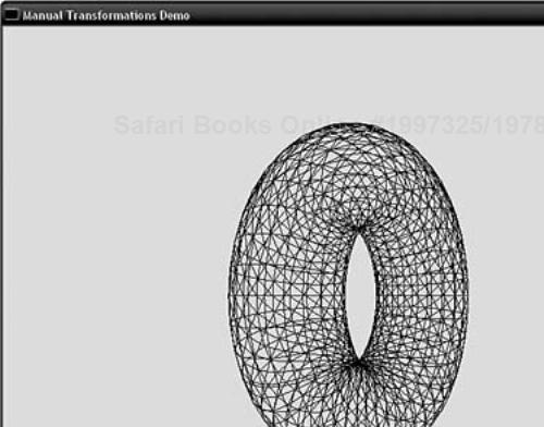
Let's look at an example now that shows how to create and load your own transformation matrix—the hard way! In the sample program TRANSFORM, we draw a torus (a doughnut-shaped object) in front of our viewing location and make it rotate in place. The function DrawTorus does the necessary math to generate the torus's geometry and takes as an argument a 4×4 transformation matrix to be applied to the vertices. We create the matrix and apply the transformation manually to each vertex to transform the torus. Let's start with the main rendering function in Listing 4.4.
Example 4.4. Code to Set Up the Transformation Matrix While Drawing
void RenderScene(void)
    {
    GLTMatrix   transformationMatrix;   // Storage for rotation matrix
    static GLfloat yRot = 0.0f;         // Rotation angle for animation
    yRot += 0.5f;

    // Clear the window with current clearing color
    glClear(GL_COLOR_BUFFER_BIT | GL_DEPTH_BUFFER_BIT);

    // Build a rotation matrix
    gltRotationMatrix(gltDegToRad(yRot), 0.0f, 1.0f, 0.0f,
                                             transformationMatrix);
    transformationMatrix[12] = 0.0f;
    transformationMatrix[13] = 0.0f;
    transformationMatrix[14] = -2.5f;

    DrawTorus(transformationMatrix);

    // Do the buffer Swap
    glutSwapBuffers();
    }
We begin by declaring storage for the matrix here:
GLTMatrix transformationMatrix; // Storage for rotation matrix
The data type GLTMatrix is of our own design and is simply a typedef declared in gltools.h for a floating-point array 16 elements long:
typedef GLfloat GLTMatrix[16]; // A column major 4x4 matrix of type GLfloat
The animation in this sample works by continually incrementing the variable yRot that represents the rotation around the y-axis. After clearing the color and depth buffer, we compose our transformation matrix as follows:
gltRotationMatrix(gltDegToRad(yRot), 0.0f, 1.0f, 0.0f, transformationMatrix);
transformationMatrix[12] = 0.0f;
transformationMatrix[13] = 0.0f;
transformationMatrix[14] = -2.5f;
Here, the first line contains a call to another glTools function, gltRotationMatrix. This function takes a rotation angle in radians (for more efficient calculations) and three arguments specifying a vector around which you want the rotation to occur. With the exception of the angle being in radians instead of degrees, this is almost exactly like the OpenGL function glRotate. The last argument is a matrix into which you want to store the resulting rotation matrix. The macro function gltDegToRad does an in-place conversion from degrees to radians.
As you saw in Figure 4.28, the last column of the matrix represents the translation of the transformation. Rather than do a full matrix multiplication, we can simply inject the desired translation directly into the matrix. Now the resulting matrix represents both a translation in space (a location to place the torus) and then a rotation of the object's coordinate system applied at that location.
Next, we pass this transformation matrix to the DrawTorus function. You do not need to list the entire function to create a torus here, but focus your attention to these lines:
objectVertex[0] = x0*r;
objectVertex[1] = y0*r;
objectVertex[2] = z;
gltTransformPoint(objectVertex, mTransform, transformedVertex);
glVertex3fv(transformedVertex);
The three components of the vertex are loaded into an array and passed to the function gltTransformPoint. This glTools function performs the multiplication of the vertex against the matrix and returns the transformed vertex in the array transformedVertex. We then use the vector version of glVertex and send the vertex data down to OpenGL. The result is a spinning torus, as shown in Figure 4.29.
It is important that you see at least once the real mechanics of how vertices are transformed by a matrix using such a drawn-out example. As you progress as an OpenGL programmer, you will find that the need to transform points manually will arise for tasks that are not specifically related to rendering operations, such as collision detection (bumping into objects), frustum culling (throwing away and not drawing things you can't see), and some other special effects algorithms.
For geometry processing, however, the TRANSFORM sample program is very inefficient. We are letting the CPU do all the matrix math instead of letting OpenGL's dedicated hardware do the work for us (which is much faster than the CPU!). In addition, because OpenGL has the modelview matrix, all our transformed points are being multiplied yet again by the identity matrix. This does not change the value of our transformed vertices, but it is still a wasted operation.
For the sake of completeness, we provide an improved example, TRANSFORMGL, that instead uses our transformation matrix but hands it over to OpenGL using the function glLoadMatrixf. We eliminate our DrawTorus function with its dedicated transformation code and use a more general-purpose torus drawing function, gltDrawTorus, from the glTools library. The relevant code is shown in Listing 4.5.
In the preceding example, we simply constructed a single transformation matrix and loaded it into the modelview matrix. This technique had the effect of transforming any and all geometry that followed by that matrix before being rendered. As you've seen in the other previous examples, we often add one transformation to another. For example, we used glTranslate followed by glRotate to first translate and then rotate an object before being drawn. Behind the scenes, when you call multiple transformation functions, OpenGL performs a matrix multiplication between the existing transformation matrix and the one you are adding or appending to it. For example, in the TRANSFORMGL example, we might replace the code in Listing 4.5 with something like the following:
glPushMatrix();
        glTranslatef(0.0f, 0.0f, -2.5f);
        glRotatef(yRot, 0.0f, 1.0f, 0.0f);

        gltDrawTorus(0.35, 0.15, 40, 20);
    glPopMatrix();
Using this approach has the effect of saving the current identity matrix, multiplying the translation matrix, multiplying the rotation matrix, and then drawing the torus by the result. You can do these multiplications yourself by using the glTools function gltMultiplyMatrix, as shown here:
GLTMatrix rotationMatrix, translationMatrix, transformationMatrix;
...
    gltRotationMatrix(gltDegToRad(yRot), 0.0f, 1.0f, 0.0f, rotationMatrix);
    gltTranslationMatrix(0.0f, 0.0f, -2.5f, translationMatrix);
    gltMultiplyMatrix(translationMatrix, rotationMatrix, transformationMatrix);
    glLoadMatrixf(transformationMatrix);

    gltDrawTorus(0.35f, 0.15f, 40, 20);
OpenGL also has its own matrix multiplication function, glMultMatrix, that takes a matrix and multiplies it by the currently loaded matrix and stores the result at the top of the matrix stack. In our final code fragment, we once again show code equivalent to the preceding, but this time we let OpenGL do the actual multiplication:
GLTMatrix rotationMatrix, translationMatrix, transformationMatrix;
...
    glPushMatrix();
       gltRotationMatrix(gltDegToRad(yRot), 0.0f, 1.0f, 0.0f, rotationMatrix);
       gltTranslationMatrix(0.0f, 0.0f, -2.5f, translationMatrix);

       glMultMatrixf(translationMatrix);
       glMultMatirxf(rotationMatrix);

    gltDrawTorus(0.35f, 0.15f, 40, 20);
   glPopMatrix();
Once again, you should remember that the glMultMatrix functions and other high-level functions that do matrix multiplication (glRotate, glScale, glTranslate) are not being performed by the OpenGL hardware, but usually by your CPU.
To represent a location and orientation of any object in your 3D scene, you can use a single 4×4 matrix that represents its transform. Working with matrices directly, however, can still be somewhat awkward, so programmers have always sought ways to represent a position and orientation in space more succinctly. Fixed objects such as terrain are often untransformed, and their vertices usually specify exactly where the geometry should be drawn in space. Objects that move about in the scene are often called actors, paralleling the idea of actors on a stage.
Actors have their own transformations, and often other actors are transformed not only with respect to the world coordinate system (eye coordinates), but with respect to other actors. Each actor with its own transformation is said to have its own frame of reference, or local object coordinate system. It is often useful to translate between local and world coordinate systems and back again for many nonrendering-related geometric tests.
A simple and flexible way to represent a frame of reference is to use a data structure (or class in C++) that contains a position in space, a vector that points forward, and a vector that points upward. Using these quantities, you can uniquely identify a given position and orientation in space. The following example from the glTools library is a GLFrame data structure that can store this information all in one place:
typedef struct{
    GLTVector3f vLocation;
    GLTVector3f vUp;
    GLTVector3f vForward;
    } GLTFrame;
Using a frame of reference such as this to represent an object's position and orientation is a very powerful mechanism. To begin with, you can use this data directly to create a 4×4 transformation matrix. Referring to Figure 4.28, the up vector becomes the y column of the matrix, whereas the forward-looking vector becomes the z column vector and the position is the translation column vector. This leaves only the x column vector, and because we know all three axes are perpendicular to one another (orthonormal), we can calculate the x column vector by performing the cross product of the y and z vectors. Listing 4.6 shows the glTools function gltGetMatrixFromFrame, which does exactly that.
Example 4.6. Code to Derive a 4×4 Matrix from a Frame
///////////////////////////////////////////////////////////////////
// Derives a 4x4 transformation matrix from a frame of reference
void gltGetMatrixFromFrame(GLTFrame *pFrame, GLTMatrix mMatrix)
    {
    GLTVector3f vXAxis;       // Derived X Axis

    // Calculate X Axis
    gltVectorCrossProduct(pFrame->vUp, pFrame->vForward, vXAxis);

    // Just populate the matrix
    // X column vector
    memcpy(mMatrix, vXAxis, sizeof(GLTVector));
    mMatrix[3] = 0.0f;

    // y column vector
    memcpy(mMatrix+4, pFrame->vUp, sizeof(GLTVector));
    mMatrix[7] = 0.0f;

    // z column vector
    memcpy(mMatrix+8, pFrame->vForward, sizeof(GLTVector));
    mMatrix[11] = 0.0f;

    // Translation/Location vector
    memcpy(mMatrix+12, pFrame->vLocation, sizeof(GLTVector));
    mMatrix[15] = 1.0f;
    }
Applying an actor's transform is as simple as calling glMultMatrixf with the resulting matrix.
Many graphics programming books recommend an even simpler mechanism for storing an object's position and orientation: Euler angles. Euler angles require less space because you essentially store an object's position and then just three angles—representing a rotation around the x-, y-, and z-axes—sometimes called yaw, pitch, and roll. A structure such as this might represent an airplane's location and orientation:
struct EULER {
    GLTVector3f    vPosition;
    GLfloat      fRoll;
    GLfloat      fPitch;
    GLfloat      fYaw;
    };
Euler angles are a bit slippery and are sometimes called “oily angles” by some in the industry. The first problem is that a given position and orientation can be represented by more than one set of Euler angles. Having multiple sets of angles can lead to problems as you try to figure out how to smoothly move from one orientation to another. Occasionally, a second problem called “gimbal lock” comes up; this problem makes it impossible to achieve a rotation around one of the axes. Lastly, Euler angles make it more tedious to calculate new coordinates for simply moving forward along your line of sight or trying to figure out new Euler angles if you want to rotate around one of your own local axes.
Some literature today tries to solve the problems of Euler angles by using a mathematical tool called quaternions. Quaternions, which can be difficult to understand, really don't solve any problems with Euler angles that you can't solve on your own by just using the frame of reference method covered previously. We already promised that this book would not get too heavy on the math, so we will not debate the merits of each system here. But we should say that the quaternion versus linear algebra (matrix) debate is more than 100 years old and by far predates their application to computer graphics!
There is really no such thing as a camera transformation in OpenGL. We use the camera as a useful metaphor to help us manage our point of view in some sort of immersive 3D environment. If we envision a camera as an object that has some position in space and some given orientation, we find that our current frame of reference system can represent both actors and our camera in a 3D environment.
To apply a camera transformation, we take the camera's actor transform and flip it so that moving the camera backward is equivalent to moving the whole world forward. Similarly, turning to the left is equivalent to rotating the whole world to the right. To render a given scene, we usually take the approach outlined in Figure 4.30.

The OpenGL utility library contains a function that uses the same data we stored in our frame structure to create our camera transformation:
void gluLookAt(GLdouble eyex, GLdouble eyey, GLdouble eyez,
        GLdouble centerx, GLdouble centery, GLdouble centerz,
        GLdouble upx, GLdouble upy, GLdouble upz);
This function takes the position of the eye point, a point directly in front of the eye point, and the direction of the up vector. The glTools library also contains a shortcut function that performs the equivalent action using a frame of reference:
Now let's work through one final example for this chapter to bring together all the concepts we have discussed so far. In the sample program SPHEREWORLD, we create a world populated by a number of spheres (Sphere World) placed at random locations on the ground. Each sphere is represented by an individual GLTFrame structure for its location and orientation. We also use the frame to represent a camera that can be moved about Sphere World using the keyboard arrow keys. In the middle of Sphere World, we use the simpler high-level transformation routines to draw a spinning torus with another sphere in orbit around it.
This example combines all the ideas we have discussed thus far and shows them working together. In addition to the main source file sphereworld.c, the project also includes the torus.c, matrixmath.c, and framemath.c modules from the glTools library found in the common subdirectory. We do not provide the entire listing here because it uses the same GLUT framework as all the other samples, but the important functions are shown in Listing 4.7.
Example 4.7. Main Functions for the SPHEREWORLD Sample
#define NUM_SPHERES      50
GLTFrame    spheres[NUM_SPHERES];
GLTFrame    frameCamera;

//////////////////////////////////////////////////////////////////
// This function does any needed initialization on the rendering
// context.
void SetupRC()
    {
    int iSphere;

    // Bluish background
    glClearColor(0.0f, 0.0f, .50f, 1.0f );

    // Draw everything as wire frame
    glPolygonMode(GL_FRONT_AND_BACK, GL_LINE);

    gltInitFrame(&frameCamera);  // Initialize the camera

    // Randomly place the sphere inhabitants
    for(iSphere = 0; iSphere < NUM_SPHERES; iSphere++)
        {
        gltInitFrame(&spheres[iSphere]);    // Initialize the frame

        // Pick a random location between -20 and 20 at .1 increments
        spheres[iSphere].vLocation[0] = (float)((rand() % 400) - 200) * 0.1f;
        spheres[iSphere].vLocation[1] = 0.0f;
        spheres[iSphere].vLocation[2] = (float)((rand() % 400) - 200) * 0.1f;
        }
    }


///////////////////////////////////////////////////////////
// Draw a gridded ground
void DrawGround(void)
    {
    GLfloat fExtent = 20.0f;
    GLfloat fStep = 1.0f;
    GLfloat y = -0.4f;
    GLint iLine;

    glBegin(GL_LINES);
       for(iLine = -fExtent; iLine <= fExtent; iLine += fStep)
          {
          glVertex3f(iLine, y, fExtent);    // Draw Z lines
          glVertex3f(iLine, y, -fExtent);

          glVertex3f(fExtent, y, iLine);
          glVertex3f(-fExtent, y, iLine);
          }

    glEnd();
    }


// Called to draw scene
void RenderScene(void)
    {
    int i;
     static GLfloat yRot = 0.0f;         // Rotation angle for animation
    yRot += 0.5f;

    // Clear the window with current clearing color
    glClear(GL_COLOR_BUFFER_BIT | GL_DEPTH_BUFFER_BIT);

    glPushMatrix();
        gltApplyCameraTransform(&frameCamera);

        // Draw the ground
        DrawGround();

        // Draw the randomly located spheres
        for(i = 0; i < NUM_SPHERES; i++)
            {
            glPushMatrix();
            gltApplyActorTransform(&spheres[i]);
            glutSolidSphere(0.1f, 13, 26);
            glPopMatrix();
            }

        glPushMatrix();
            glTranslatef(0.0f, 0.0f, -2.5f);

            glPushMatrix();
                glRotatef(-yRot * 2.0f, 0.0f, 1.0f, 0.0f);
                glTranslatef(1.0f, 0.0f, 0.0f);
                glutSolidSphere(0.1f, 13, 26);
            glPopMatrix();

            glRotatef(yRot, 0.0f, 1.0f, 0.0f);
            gltDrawTorus(0.35, 0.15, 40, 20);
        glPopMatrix();
    glPopMatrix();

    // Do the buffer Swap
    glutSwapBuffers();
    }


// Respond to arrow keys by moving the camera frame of reference
void SpecialKeys(int key, int x, int y)
    {
    if(key == GLUT_KEY_UP)
        gltMoveFrameForward(&frameCamera, 0.1f);

    if(key == GLUT_KEY_DOWN)
        gltMoveFrameForward(&frameCamera, -0.1f);

    if(key == GLUT_KEY_LEFT)
        gltRotateFrameLocalY(&frameCamera, 0.1);

    if(key == GLUT_KEY_RIGHT)
        gltRotateFrameLocalY(&frameCamera, -0.1);

    // Refresh the Window
    glutPostRedisplay();
    }
The first few lines contain a macro to define the number of spherical inhabitants as 50. Then we declare an array of frames and another frame to represent the camera:
#define NUM_SPHERES      50
GLTFrame    spheres[NUM_SPHERES];
GLTFrame    frameCamera;
The SetupRC function calls the glTools function gltInitFrame on the camera to initialize it as being at the origin and pointing down the negative z-axis (the OpenGL default viewing orientation):
gltInitFrame(&frameCamera); // Initialize the camera
You can use this function to initialize any frame structure, or you can initialize the structure yourself to have any desired position and orientation. Next, a loop initializes the array of sphere frames and selects a random x and z location for their positions:
// Randomly place the sphere inhabitants
    for(iSphere = 0; iSphere < NUM_SPHERES; iSphere++)
        {
        gltInitFrame(&spheres[iSphere]);    // Initialize the frame

        // Pick a random location between -20 and 20 at .1 increments
        spheres[iSphere].vLocation[0] = (float)((rand() % 400) - 200) * 0.1f;
        spheres[iSphere].vLocation[1] = 0.0f;
        spheres[iSphere].vLocation[2] = (float)((rand() % 400) - 200) * 0.1f;
        }
The DrawGround function then draws the ground as a series of criss-cross grids using a series of GL_LINE segments:
///////////////////////////////////////////////////////////
// Draw a gridded ground
void DrawGround(void)
    {
    GLfloat fExtent = 20.0f;
    GLfloat fStep = 1.0f;
    GLfloat y = -0.4f;
    GLint iLine;

    glBegin(GL_LINES);
       for(iLine = -fExtent; iLine <= fExtent; iLine += fStep)
          {
          glVertex3f(iLine, y, fExtent);    // Draw Z lines
          glVertex3f(iLine, y, -fExtent);

          glVertex3f(fExtent, y, iLine);
          glVertex3f(-fExtent, y, iLine);
          }

    glEnd();
    }
The RenderScene function draws the world from our point of view. Note that we first save the identity matrix and then apply the camera transformation using the glTools helper function gltApplyCameraTransform. The ground is static and is transformed by the camera only to appear that you are moving over it:
glPushMatrix();
        gltApplyCameraTransform(&frameCamera);

        // Draw the ground
        DrawGround();
Then we draw each of the randomly located spheres. The gltApplyActorTransform function creates a transformation matrix from the frame of reference and multiplies it by the current matrix (which is the camera matrix). Each sphere must have its own transform relative to the camera, so the camera is saved each time with a call to glPushMatrix and restored again with glPopMatrix to get ready for the next sphere or transformation:
// Draw the randomly located spheres
for(i = 0; i < NUM_SPHERES; i++)
    {
    glPushMatrix();
    gltApplyActorTransform(&spheres[i]);
    glutSolidSphere(0.1f, 13, 26);
    glPopMatrix();
    }
Now for some fancy footwork! First, we move the coordinate system a little further down the z-axis so that we can see what we are going to draw next. We save this location and then perform a rotation, followed by a translation and the drawing of a sphere. This effect makes the sphere appear to revolve around the origin in front of us. We then restore our transformation matrix, but only so that the location of the origin is z = –2.5. Then another rotation is performed before the torus is drawn. This has the effect of making a torus that spins in place:
    glPushMatrix();
        glTranslatef(0.0f, 0.0f, -2.5f);

        glPushMatrix();
            glRotatef(-yRot * 2.0f, 0.0f, 1.0f, 0.0f);
            glTranslatef(1.0f, 0.0f, 0.0f);
            glutSolidSphere(0.1f, 13, 26);
        glPopMatrix();

        glRotatef(yRot, 0.0f, 1.0f, 0.0f);
        gltDrawTorus(0.35, 0.15, 40, 20);
    glPopMatrix();
glPopMatrix();
The total effect is that we see a grid on the ground with many spheres scattered about at random locations. Out in front, we see a spinning torus, with a sphere moving rapidly in orbit around it. Figure 4.31 shows the result.

Finally, the SpecialKeys function is called whenever one of the arrow keys is pressed. The up-and down-arrow keys call the glTools function gltMoveFrameForward, which simply moves the frame forward along its line of sight. The gltRotateFrameLocalY function rotates a frame of reference around its local y-axis (regardless of orientation) in response to the left-and right-arrow keys:
void SpecialKeys(int key, int x, int y)
    {
    if(key == GLUT_KEY_UP)
        gltMoveFrameForward(&frameCamera, 0.1f);

    if(key == GLUT_KEY_DOWN)
        gltMoveFrameForward(&frameCamera, -0.1f);

    if(key == GLUT_KEY_LEFT)
        gltRotateFrameLocalY(&frameCamera, 0.1);

    if(key == GLUT_KEY_RIGHT)
        gltRotateFrameLocalY(&frameCamera, -0.1);

    // Refresh the Window
    glutPostRedisplay();
    }
In this chapter, you learned concepts crucial to using OpenGL for creation of 3D scenes. Even if you can't juggle matrices in your head, you now know what matrices are and how they are used to perform the various transformations. You also learned how to manipulate the modelview and projection matrix stacks to place your objects in the scene and to determine how they are viewed onscreen.
We also showed you the functions needed to perform your own matrix magic, if you are so inclined. These functions allow you to create your own matrices and load them on to the matrix stack or multiply them by the current matrix first. The chapter also introduced the powerful concept of a frame of reference, and you saw how easy it is to manipulate frames and convert them into transformations.
Finally, we began to make more use of the glTools library that accompanies this book. This library is written entirely in portable ANSI C and provides you with a handy toolkit of miscellaneous math and helper routines that can be used along with OpenGL.
glLoadIdentity | |
|---|---|
Purpose: | |
Include File: |
|
Syntax: | |
void glLoadIdentity(void); | |
Description: | This function replaces the current transformation matrix with the identity matrix. This essentially resets the coordinate system to eye coordinates. |
Returns: | None. |
See Also: |
|
glMatrixMode | |
|---|---|
Purpose: | Specifies the current matrix ( |
Include File: |
|
Syntax: | |
void glMatrixMode(GLenum mode );
| |
Description: | This function determines which matrix stack ( |
Parameters: | |
|
|
Table 4.2. Valid Matrix Mode Identifiers for glMatrixMode
Mode | Matrix Stack |
|---|---|
| Matrix operations affect the modelview matrix stack. (Used to move objects around the scene.) |
| Matrix operations affect the projection matrix stack. (Used to define clipping volume.) |
| Matrix operations affect the texture matrix stack. (Manipulates texture coordinates.) |
Returns: | None. |
See Also: |
|
glPopMatrix | |
|---|---|
Purpose: | |
Include File: |
|
Syntax: | |
void glPopMatrix(void); | |
Description: | This function pops the last (topmost) matrix off the current matrix stack. This function is most often used to restore the previous condition of the current transformation matrix if it was saved with a call to |
Returns: | None. |
See Also: |
|
gluLookAt | |
|---|---|
Purpose: | |
Include File: |
|
Syntax: | |
void gluLookAt(GLdouble eyex, GLdouble eyey, | |
Description: | Defines a viewing transformation based on the position of the eye, the position of the center of the scene, and a vector pointing up from the viewer's perspective. |
Parameters: | |
| |
|
|
|
|
Returns: | None. |
See Also: |
|
gluPerspective | |
|---|---|
Purpose: | |
Include File: |
|
Syntax: | |
void gluPerspective(GLdouble fovy, GLdouble aspect | |
Description: | This function creates a matrix that describes a viewing frustum in world coordinates. The aspect ratio should match the aspect ratio of the viewport (specified with |
Parameters: | |
| |
|
|
|
|
Returns: | None. |
See Also: |
|