Appendix The Basics of SQL

Structured Query Language, or SQL, is the ISO-ANSI standard data definition and manipulation language for relational database management systems. Individual relational database systems use slightly different dialects of SQL syntax and naming rules, and these differences can be seen in the SQL user guides for those systems. In this text, as we explore each step of the logical and physical design portion of the database life cycle, many examples of database table creation and manipulation make use of SQL syntax.

Basic SQL use can be learned quickly and easily by reading this appendix. The more advanced features, such as statistical analysis and presentation of data, require additional study and are beyond the reach of the typical nonprogrammer. However, the DBA can create SQL views to help nonprogrammers set up repetitive queries; other languages, such as forms, are being commercially sold for nonprogrammers. For the advanced database programmer, embedded SQL (in C programs, for instance) is widely available for the most complex database applications, which need the power of procedural languages.

This appendix introduces the reader to the basic constructs for the SQL-99 (and SQL-92) database definition, queries, and updates through a sequence of examples with some explanatory text. We start with a definition of SQL terminology for data types and operators. This is followed by an explanation of the data definition language (DDL) constructs using the “create table” commands, including a definition of the various types of integrity constraints, such as foreign keys and referential integrity. Finally, we take a detailed look at the SQL-99 data manipulation language (DML) features through a series of simple and then more complex practical examples of database queries and updates.

The specific features of SQL, as implemented by the major vendors IBM, Oracle, and Microsoft, can be found in the references at the end of this appendix.

A.1 SQL Names and Operators

This section gives the basic rules for SQL-99 (and SQL-92) data types and operators.

• SQL names: Although these have no particular restrictions, some vendor-specific versions of SQL do have some restrictions. For example, in Oracle, names of tables and columns (attributes) can be up to 30 characters long, must begin with a letter, and can include the symbols (a-z, 0-9, _, $, #). Names should not duplicate reserved words or names for other objects (attributes, tables, views, indexes) in the database.
• Data types for attributes: character, character varying, numeric, decimal, integer, smallint, float, double precision, real, bit, bit varying, date, time, timestamp, interval.
• Logical operators: and, or, not, ().
• Comparison operators: =, <>, <, <=, >, »=, (), in, any, some, all, between, not between, is null, is not null, like.
• Set operators:

— union: combines queries to display any row in each subquery

— intersect: combines queries to display distinct rows common to all subqueries

— except: combines queries to return all distinct rows returned by the first query, but not the second (this is “minus” or “difference” in some versions of SQL)

• Set functions: count, sum, min, max, avg.
• Advanced value expressions: CASE, CAST, row value constructors. CASE is similar to CASE expressions in programming languages, in which a select command needs to produce different results when there are different values of the search condition. The CAST expression allows you to convert data of one type to a different type, subject to some restrictions. Row value constructors allow you to set up multiple column value comparisons with a much simpler expression than is normally required in SQL (see Melton and Simon [1993] for detailed examples).

A.2 Data Definition Language (DDL)

The basic definitions for SQL objects (tables and views) are:

• create table: defines a table and all its attributes
• alter table: add new columns, drop columns, or modifies existing columns in a table
• drop table: deletes an existing table
• create view, drop view: defines/deletes a database view (see Section A.3.4)

Some versions of SQL also have create index/drop index, which defines/deletes an index on a particular attribute or composite of several attributes in a particular table.

The following table creation examples are based on a simple database of three tables: customer, item, and order. (Note that we put table names in boldface throughout the book for readability.)

Note that the attribute cust_num could be defined as “numeric not null unique” instead of explicity defined as the primary key, since they both have the same meaning. However, it would be redundant to have both forms in the same table definition. The check rule is an important integrity constraint that tells SQL to automatically test each insertion of credit_level value for something greater than or equal to 1000. If not, an error message should be displayed.

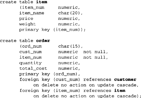
SQL, while allowing the above format for primary key and foreign key, recommends a more detailed format, shown below, for table order:

in which pk_constr is a primary key constraint name, and fk_constr1 and fk_constr2 are foreign key constraint names. The word “constraint” is a keyword, and the object in parentheses after the table name is the name of the primary key in that table referenced by the foreign key.

The following constraints are common for attributes defined in the SQL create table commands:

• Not null: a constraint that specifies that an attribute must have a nonnull value.
• Unique: a constraint that specifies that the attribute is a candidate key; that is, that it has a unique value for every row in the table. Every attribute that is a candidate key must also have the constraint not null. The constraint unique is also used as a clause to designate composite candidate keys that are not the primary key. This is particularly useful when transforming ternary relationships to SQL.
• Primary key: the primary key is a set of one or more attributes that, when taken collectively, enables us to uniquely identify an entity or table. The set of attributes should not be reducible (see Section 6.1.2). The designation primary key for an attribute implies that the attribute must be not null and unique, but the SQL keywords NOT NULL and UNIQUE are redundant for any attribute that is part of a primary key, and need not be specified in the create table command.
• Foreign key: the referential integrity constraint specifies that a foreign key in a referencing table column must match an existing primary key in the referenced table. The references clause specifies the name of the referenced table. An attribute may be both a primary key and a foreign key, particularly in relationship tables formed from many-to-many binary relationships or from n-ary relationships.

Foreign key constraints are defined for deleting a row on the referenced table and for updating the primary key of the referenced table. The referential trigger actions for delete and update are similar:

• on delete cascade: the delete operation on the referenced table “cascades” to all matching foreign keys.
• on delete set null: foreign keys are set to null when they match the primary key of a deleted row in the referenced table. Each foreign key must be able to accept null values for this operation to apply.
• on delete set default: foreign keys are set to a default value when they match the primary key of the deleted row(s) in the reference table. Legal default values include a literal value, “user,” “system user,” or “no action.”
• on update cascade: the update operation on the primary key(s) in the referenced table “cascades” to all matching foreign keys.
• on update set null: foreign keys are set to null when they match the old primary key value of an updated row in the referenced table. Each foreign key must be able to accept null values for this operation to apply.
• on update set default: foreign keys are set to a default value when they match the primary key of an updated row in the reference table. Legal default values include a literal value, “user,” “system user,” or “no action.”

The cascade option is generally applicable when either the mandatory existence constraint or the ID dependency constraint is specified in the ER diagram for the referenced table, and either set null or set default is applicable when optional existence is specified in the ER diagram for the referenced table (see Chapters 2 and 5).

Some systems, such as DB2, have an additional option on delete or update, called restricted. Delete restricted means that the referenced table rows are deleted only if there are no matching foreign key values in the referencing table. Similarly, update restricted means that the referenced table rows (primary keys) are updated only if there are no matching foreign key values in the referencing table.

Various column and table constraints can be specified as deferrable (the default is not deferrable), which means that the DBMS will defer checking this constraint until you commit the transaction. Often this is required for mutual constraint checking.

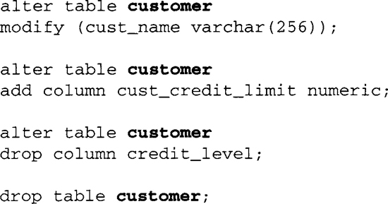
The following examples illustrate the alter table and drop table commands. The first alter table command modifies the cust_name data type from char(20) in the original definition to varchar(256). The second and third alter table commands add and drop a column, respectively. The add column option specifies the data type of the new column.

A.3 Data Manipulation Language (DML)

Data manipulation language commands are used for queries, updates, and the definition of views. These concepts are presented through a series of annotated examples, from simple to moderately complex.

A.3.1 SQL Select Command

The SQL select command is the basis for all database queries. The following series of examples illustrates the syntax and semantics of the select command for the most frequent types of queries in everyday business applications. To illustrate each of the commands, we assume the following set of data in the database tables:

Basic Commands

This results in a display of the complete customer table (as shown above).

Union and Intersection Commands

Aggregate Functions

Joins and Subqueries

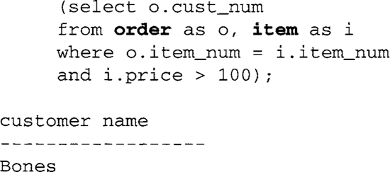
This query can be equivalently performed with a subquery (sometimes called a nested subquery) with the following format. The select command inside the parentheses is a nested subquery and is executed first, resulting in a set of values for customer number (cust_num) selected from the order table. Each of those values is compared with cust_num values from the customer table, and matching values result in the display of customer name from the matching row in the customer table. This is effectively a join between tables customer and order with the selection condition of item number 125.

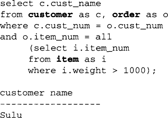
Note that Kirk has ordered one item weighing over 1000 (starShip), but he has also ordered an item weighing under 1000 (captainsLog), so his name does not get displayed.

A.3.2 SQL Update Commands

The following SQL update commands relate to our continuing example and illustrate typical usage of insertion, deletion, and update of selected rows in tables.

This command adds one more customer (klingon) to the customer table:

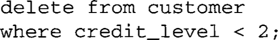
This command deletes all customers with credit levels less than 2:

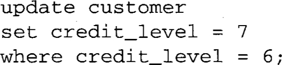
This command modifies the credit level of any customer with level 6 to level 7:

A.3.3 Referential Integrity

The following update to the item table resets the value of item_num for a particular item, but because item_num is a foreign key in the order table, SQL must maintain referential integrity by triggering the execution sequence named by the foreign key constraint on update cascade in the definition of the order table (see Section A2). This means that, in addition to updating a row in the item table, SQL will search the order table for values of item_num equal to 368 and reset each item_num value to 370.

If this update had been a delete instead, such as the following:

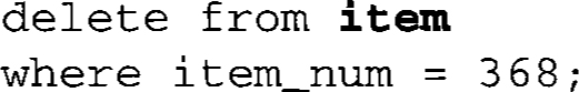
then the referential integrity trigger would have caused the additional execution of the foreign key constraint on delete set default in order (as defined in Section A.2), which finds every row in order with item_num equal to 368 and takes the action set up in the default. A typical action for this type of database might be to set item_num to either null or a predefined literal value to denote that the particular item has been deleted; this would then be a signal to the system that the customer needs to be contacted to change the order. Of course, the system would have to be set up in advance to check for these values periodically.

A.3.4 SQL Views

A view in SQL is a named, derived (virtual) table that derives its data from base tables, the actual tables defined by the create table command. View definitions can be stored in the database, but the views (derived tables) themselves are not stored; they are derived at execution time when the view is invoked as a query using the SQL select command. The person who queries the view treats the view as if it were an actual (stored) table, unaware of the difference between the view and the base table.

Views are useful in several ways. First, they allow complex queries to be set up in advance in a view, and the novice SQL user is only required to make a simple query on the view. This simple query invokes the more complex query defined by the view. Thus, nonprogrammers are allowed to use the full power of SQL without having to create complex queries. Second, views provide greater security for a database, because the DBA can assign different views of the data to different users and control what any individual user sees in the database. Third, views provide a greater sense of data independence; that is, even though the base tables may be altered by adding, deleting, or modifying columns, the view query may not need to be changed. While view definition may need to be changed, that is the job of the DBA, not the person querying the view.

Views may be defined hierarchically; that is, a view definition may contain another view name as well as base table names. This enables some views to become quite complex.

In the following example, we create a view called “orders” that shows which items have been ordered by each customer and how many. The first line of the view definition specifies the view name and (in parentheses) lists the attributes of that view. The view attributes must correlate exactly with the attributes defined in the select statement in the second line of the view definition:

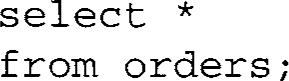
The create view command creates the view definition, which defines two joins among three base tables customer, item, and order; and SQL stores the definition to be executed later when invoked by a query. The following query selects all the data from the view “orders.” This query causes SQL to execute the select command given in the preceding view definition, producing a tabular result with the column headings for customer_name, item_name, and quantity.

Usually, views are not allowed to be updated, because the updates would have to be made to the base tables that make up the definition of the view. When a view is created from a single table, the view update is usually unambiguous, but when a view is created from the joins of multiple tables, the base table updates are very often ambiguous and may have undesirable side effects. Each relational system has its own rules about when views can and cannot be updated.

A.4 References

Bulger B., Greenspan, J., and Wall, D. MySQL/PHP Database Applications, 2nd ed., Wiley, 2004.

Gennick, J. Oracle SQL*Plus: The Definitive Guide, O’Reilly, 1999.

Gennick, J. SQL Pocket Guide, O’Reilly, 2004.

Melton, J., and Simon, A. R. Understanding The New SQL: A Complete Guide, Morgan Kaufmann, 1993.

Mullins, C. S. DB2 Developer’s Guide, 5th ed., Sams Publishing, 2004.

Neilson, P. Microsoft SQL Server Bible, Wiley, 2003.

van der Lans, R. Introduction to SQL: Mastering the Relational Database Lannguage, 3rd ed., Addison-Wesley, 2000.