
Effective FPV for verification
In this chapter we describe how to effectively use FPV for two main types of design verification: bug hunting, where we supplement simulation to try to find tricky corner case bugs; and full proof FPV, where we try to fully establish that an RTL design implements a desired specification. Using the example of a simple Arithmetic Logic Unit (ALU) design, we then show how to create a plan for bug hunting FPV on this model, exploring and expanding upon the parallels with the design exercise FPV discussed in the previous chapter. We walk through the process of planning, wiggling, and expanding FPV verification, in order to be able to gain confidence that we have verified the basic requirements of our logic, and prevented common errors that would cause incomplete coverage. Finally, we discuss changes that would be required to advance from bug hunting to full proof FPV on this model.
Keywords
FPV; bug hunting; full proof; wiggling; complexity staging
[With formal verification,] people are able to take designs, plan about what they can verify in a design, while they are building a test bench run regressions, measure progress, measure coverage, and in the end check off and sign off and say we are completely done.
Vigyan Singhal, Oski Technologies
Now that we have explored the basic methods of formal verification (FV) through design exercise, we are well poised to discuss and explore more validation-oriented modes of formal property verification (FPV). In the previous chapter, we explored the power of formal technology and observed how design exercise can help users to better understand their register transfer level (RTL) designs. In this chapter, we are going to dive into a couple of more advanced design verification techniques: bug hunting FPV and full proof FPV. The bug hunting mode of FPV is typically applied on a reasonably complex block where complimentary validation methods such as simulation or emulation are expected to be used as well. The goal of FPV on such a block would be to target complex scenarios and discover subtle corner cases that are unlikely to be hit through simulation. Full proof FPV, the traditional goal of the original FPV research pioneers, generally targets complex or risky designs with an intention to completely prove that the design meets its specification. If done properly, full proof FPV can be used to completely replace unit-level simulation testing.
When planning validation-focused FPV, you need to decide on your goals: whether to use it to supplement other forms of validation and hunt for bugs, or to use as the primary method of validation and completely verify the design formally. If you are inexperienced with FPV, we usually recommend that you start with RTL exercise, then advance to a bug hunting effort and choose whether to expand to full proof based on your initial level of success. After some experience, you should be better able to judge which mode of FPV suits your design best.
The remainder of this chapter describes the practical issues in setting up a robust FPV environment and effectively using it on your model for bug hunting and full proof scenarios. This includes a good understanding of the extended wiggling process, to refine your assumptions iteratively, and build a strong FPV environment. You will also need to think about coverage issues and to include the use of good cover points to justify that you are truly verifying your interesting design space. We illustrate this process on an example design to provide a direct demonstration of our major points.
Deciding on Your FPV Goals
First, if you are thinking about validation-focused FPV, you need to make sure you choose an appropriate design style to work with. FPV is most effective on control logic blocks, or data transport blocks. By “data transport,” we mean a block that essentially routes data from one point to another. This contrasts with “data transformation” blocks, which perform complex operations on the data, such as floating point arithmetic or MPEG decoder logic: most FPV tools cannot handle these well. Light arithmetic operations, such as integer addition and subtraction, are often acceptable for the current generation of tools, but you will probably need other forms of validation for major blocks involving multiplication, division, or floating point methods.
Before we embark on deciding the FPV goal for the design under test (DUT), we need to understand more clearly what we mean by bug hunting FPV and full proof FPV.
Bug Hunting FPV
Bug hunting FPV is a technique to hunt for potential corner-case issues in a design that we might miss through other techniques. The most important design requirements are written as assertions, and you prove that illegal assertion-violating conditions are not possible, or use the FPV tool to discover the existence of such scenarios in the design. This method is typically used if part of your design is seen as especially risky due to large number of corner cases and you want extra confidence in your verification even after running your full set of random simulations. It is common to resort to bug hunting FPV when hitting simulation coverage problems at a late design stage to ensure that there are not any tricky corner cases waiting to be exposed.
Some of the common situations that would lead you to choose bug hunting FPV are as follows:
• You are working on a design containing many corner cases, such as a large piece of control logic with several interacting state machines, and want an extra level of validation confidence.
• You have been running regular simulations on your design, and some part of it repeatedly exposes new errors during random tests.
• You are verifying a critical component of your design, and similar blocks have a history of logic bugs escaping to late stages or to silicon.
• You have already done design exercise FPV on your model, so increasing your FPV coverage by adding additional targeted assertions has a relatively low cost.
• You have a mature/reused model that mostly does not need further verification, but you have added a new feature that you want to verify with confidence.
• You have a bug that was found with a random test in a higher-level simulation testbench and you are finding it tough to reproduce the same bug at unit level because you would need a complex and rare set of input conditions.
Here, FPV is used as supplement to simulation. You are free to allow some level of overconstraining or some other compromises, as discussed in the design exercise context in the previous chapter. Don’t shy away from adding constraints that limit you to exercise only a part of the complete set of possible behaviors, the part you wish to focus on, or where you suspect a lurking bug. This is absolutely acceptable when you are doing bug hunting FPV.
This is a medium effort activity, more effort intensive than design exercise FPV but simpler than full proof FPV, and can function as a decent compromise between the other two forms.
Full Proof FPV
Full proof FPV is the usage model that corresponds most closely with the original motivation for FV research: generating solid proofs that your design is 100% correct. Full proof FPV is a high-effort activity, as it involves trying to prove the complete functionality of the design. As a result, the return on such investment is high as well: you can use it as a substitute for unit-level simulation. Thus, you can save the effort you would have spent on running simulations or other validation methods. A design completely proven through FPV, with a solid set of assertions to fully define the specification, along with solid and well-reviewed sets of cover points and assumptions, provides as much or more confidence than many months of random regressions on a full simulation environment. This method also reduces the risk of hard-to-find misses and nightmares due to corner-case behaviors not anticipated during test planning, which are often experienced in late stages of traditional validation.
You should consider running full proof FPV on your RTL if:
• You are provided with a detailed reference specification that is expected to be implemented.
• You have a design that conforms to standard interfaces where packages of pre-verified FPV collateral are available or the set of needed constraints is clearly documented.
• Your design is defined by a set of tables that fully encapsulate the expected behavior.
• You have a part of your RTL that needs bulletproof verification to reduce design risk.
• You have completed an initial effort at bug hunting FPV, and it was successful enough that you believe you can expand your assertion set and reduce your overconstraints to cover the full specification.
• You have successfully run full proof FPV on similar blocks in the past and are confident you can develop a similar verification plan.
Staging Your FPV Efforts
Because full proof FPV can be a substantial effort, we always recommend that you start with design exercise FPV, expand it into bug hunting, and gradually march toward the full proof mode. Your design exercise will function as an initial sanity-check that you have chosen a design whose size is appropriate for FPV, and whose logic is of a complexity level that is reasonable for FPV tools to handle. As we discussed in the previous chapter, design exercise enables you to do a relatively lightweight planning effort, and quickly get some hands-on results that will give you confidence in the tool’s ability to handle your design. Once you observe decent results by extensive wiggling, are confident about the environment you created, and are satisfied that you have fulfilled the goals in your design exercise plan, it is time to transition to bug hunting.
When ready to begin bug hunting, you should begin by creating a bug hunting verification plan. Once you have created this plan, start adding more complex assertions to the design and verify them, doing further wiggling, improving your modeling, and refining constraints as needed. It is perfectly fine to have your design overconstrained in the bug hunting mode, though you will often be gradually removing those constraints to find larger classes of bugs. After you have achieved the goals in your bug hunting plan, it is time to consider full proof FPV.
When planning full proof FPV, you need to be very careful about the full coverage of the design. Make sure you are starting with a solid specification document (or demand one from your architects), and be sure that your planning includes not only a full set of assertions, but also a broad set of cover points that can instill confidence in the verification effort spent. There is always an issue of logical holes lurking—some of which you would have never thought of if not examining cover points. In some cases, commercial tool features can help with coverage information as well. But even when you have tool features to help check coverage, you need to carefully think through the needed set of cover points: no tool can completely substitute for human design intuition.
Now we will look more into the steps involved in achieving your FPV goals, as we walk through the core ideas of bug hunting FPV on the basis of a simple arithmetic logic unit (ALU) design example.
Example for this Chapter: Simple ALU
For our illustration of design exercise FPV, we resort to yet another common example in the formal world, a simple ALU. As in our other examples, we use a simple design with some intentional flaws to illustrate the usage of FPV—no guarantees that it would not create another FDIV bug.
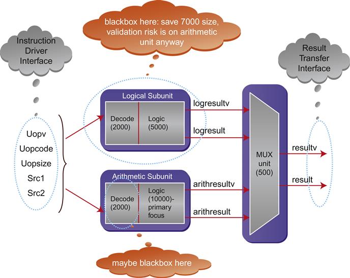
Figure 6.1 illustrates the basic block diagram of the ALU under consideration, with a few simple requirements in the specification:
• The logical unit computes simple logical operations: OR, AND, and NOT.
• The arithmetic unit computes simple arithmetic computations: addition, subtraction, and compare.
• The results are accompanied by the respective valid signals logresultv/arithresultv and the final selection to the output is based on the operation.
• The computation takes three clocks to produce results at the output ports.
• There are four threads running in parallel computing on a large vector; in other words, the below logic is replicated four times.

(The full SystemVerilog model can be downloaded from the book website at http://formalverificationbook.com if you would like to try it yourself.)
You can see from Figure 6.1 that the operations are computed in parallel and hence there is an opportunity for simple power savings that is embedded as a part of the design. Only the selected computation logic is active, while the other portion of the unit can be effectively clock-gated, cut off from the clock lines to prevent logic transitions and reduce overall power usage. The top-level code for this design is shown in Figure 6.2.
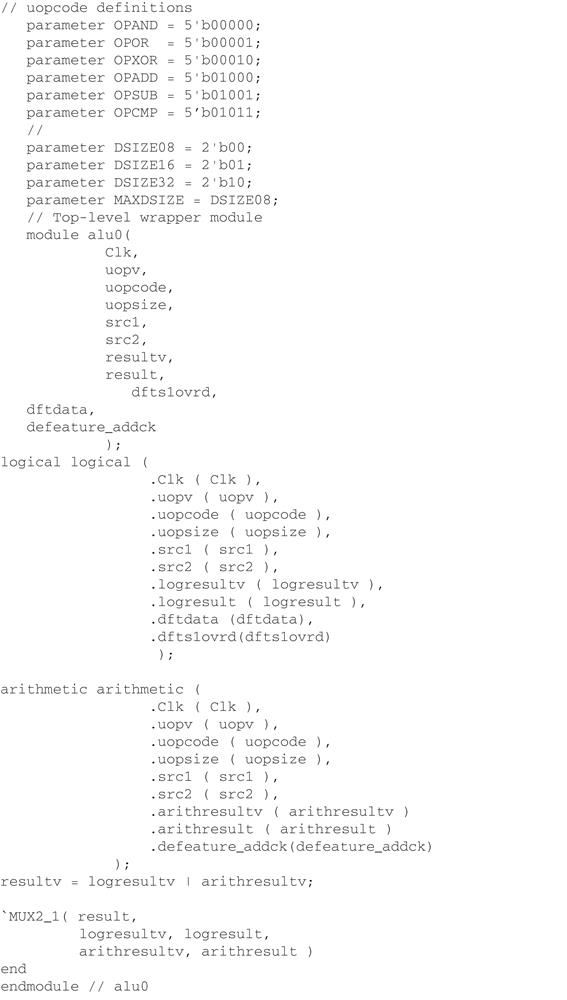
For brevity, only the instantiations and final connections are depicted here. The ALU considered here also has debug-related signals that are not shown in the above code. The μops (micro-operations) can operate on three different data sizes (DSIZE), whose encodings are also defined.
Understanding the Design
Remember that before you enter a validation-focused FPV effort, whether bug hunting or full proof, you should begin with design exercise FPV, as we discussed in the previous chapter. This will play a critical role in helping to judge the general feasibility of FPV on the chosen design, based on a lightweight initial effort. For the remainder of this discussion, we will assume that design exercise FPV has already been completed on the ALU, and we are looking to expand our efforts into bug hunting and eventually to full proof FPV.
When transitioning from design exercise to bug hunting FPV, the first step is identifying the right DUT block for verification. As we have discussed in previous chapters, FPV tools have a fundamental limitation on the amount of logic they can meaningfully consume to provide verification feedback. This is because, by very definition, the formal tools explore all possible behaviors exhibited by design block being tested, which is a computationally expensive problem. In addition, the performance of FPV engines can vary widely based on the internal structure of the logic, independent of model size, so it is best to avoid pushing against the maximum capacity of the engines when it can be avoided. Thus we should not feed the formal tools arbitrarily large design blocks to test.
To make the best use of the tool’s limited capacity, we carve out the most interesting parts of a design when choosing our DUT. There needs to be a good balance between having the flexibility in choosing an arbitrary piece of logic and choosing a DUT that is large enough and well-documented enough that creating a verification plan is clear.
In the case of our ALU example, the design contains four parallel copies of the ALU, one for each thread. But if our primary focus is on the ALU functionality, rather than the thread dispatching logic at the top level, it probably makes the most sense for us to focus on the ALU logic itself, verifying one single generic ALU instance rather than the top-level model that has four of them. This provides us significant potential complexity savings, with one quarter the logic to analyze of the full model.
The number of state elements we describe may sound somewhat limiting, but keep in mind that in most cases you will be blackboxing large embedded memories, as we will discuss in the complexity section below.
Once you have identified the DUT that you are choosing for the bug hunting effort, the next step is to make sure you have a good understanding of your model. You should start by looking at a block diagram of your proposed initial DUT, and by doing the following:
• Determine the approximate sizes, in number of state elements, for each major submodule. Many EDA tools can display this information for compiled models.
• Identify the blocks you would like to target with FPV. Remember to consider both the design sizes and the style of logic: control logic or data transport blocks tend to work best with FPV tools.
• Identify blackbox candidates: submodules that you might be able to eliminate from consideration if needed. Try to blackbox blocks whose logic is least likely to meaningfully affect your primary targets. You also need to think about the potential effort required to create interface assumptions that model that block’s output behavior, if it affects your targets.
• Identify major external interfaces that need to be properly constrained.
The above items are not always very easy to determine, of course. If you have simulation waveforms available from the current design or a similar design from a previous project, you should also examine them for guidance. These waveforms can help you determine which parts of your interfaces are active during typical transactions, and whether critical activity takes place on the interfaces of your proposed blackboxes.
For our ALU, we would probably generate a diagram something like Figure 6.3. Here we are assuming that the arithmetic logic has been identified as a primary risk area, so we want to be sure that our FPV environment ultimately tests this logic.
Once we have generated this diagram and understand the basic design flow, blocks, and interfaces of our model, it is time to work on the bug hunting FPV plan.
Creating the FPV Verification Plan
Let’s assume that we have chosen to undertake FPV because we want to exhaustively check the corner cases of the arithmetic logic and achieve more confidence in the functionality of the design. We should try to start with:
• A clear understanding of our goals.
• The kinds of properties we will be looking at, including cover points that should be hit.
• A staging plan for how to initially overconstrain the verification and gradually remove the overconstraints.
• A decomposition strategy to be deployed, if needed, to deal with the level of complexity.
• Success criteria for determining when we have done sufficient FPV.
The verification plan is subject to change; you should be able to take the feedback from the initial FPV runs and tune your plan to drive the rest of the verification effort. The plan should be easily translatable to the FPV environment, which would involve creating properties that could be constraints (assumptions), functional checks (assertions), and sanity-checkers (covers). Don’t be surprised to see this refinement loop being executed many times, as new issues and learnings are uncovered, which motivate fine-tuning the verification plan and the FPV environment. At all stages, the cover points help you to continuously sanity-check that you are still observing interesting activity in your design.
FPV Goals
One of the main goals of bug hunting FPV is to expose the corner-case issues that would be hard to hit through simulations. To better enable the examination of corner cases, we should try to create properties involving each of the major functions of our design, or of the part of our design we consider to have the greatest risk. For the ALU example in this chapter, we might consider verifying all opcodes for a specific class of operations and specific cases of DSIZE, while in full proof mode we would consider all the cases: the cross-product of all DSIZEs and all opcodes.
Most of the design behaviors would be defined in the specification document. If doing bug hunting FPV, we can use this as a guide to the most important features. If doing full proof FPV, we should carefully review this document, and make sure its requirements have been included in our FPV plan.
Based on the considerations above, we can come up with the initial set of goals for our bug hunting FPV on the ALU:
• Verify the behavior of the arithmetic unit, in the absence of any unusual activity such as power-gating or scan/debug hooks, for the default DSIZE 08.
• If time permits, expand to check the logical operators as well and additional DSIZE values.
• Once all the above checks are complete, consider adding checks for the power-gating and scan/debug features.
Major Properties for FPV
As per the verification plan, you should decide on the major properties you want to include in your FPV environment. At this point we should describe the properties in plain English for planning purposes; the real coding in SystemVerilog Assertions (SVA) will follow later.
Cover points
As explained earlier, for any FPV activity, the cover points are the most critical properties at early stages. We begin with writing covers of typical activity and interesting combinations of basic behaviors. We would start with defining a cover property for each opcode and flow that was described in waveforms in the specification document.
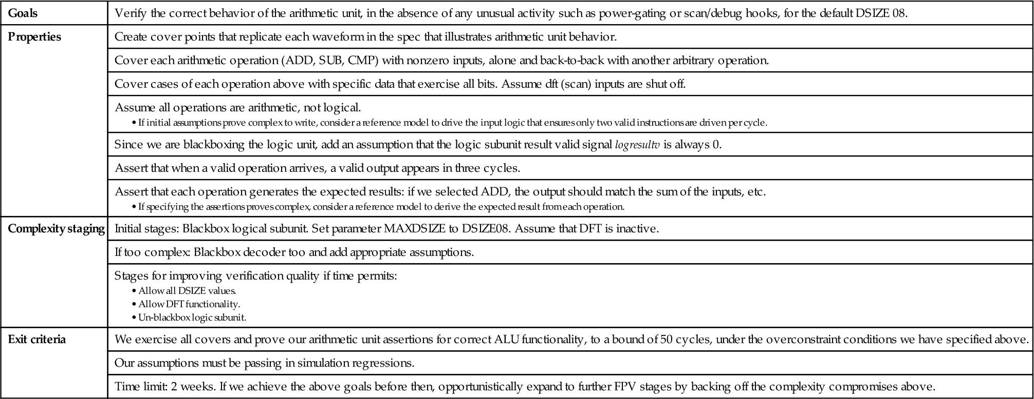
Figure 6.4 shows an example of a waveform that might appear in our specification, demonstrating the flow of arithmetic and logic operations, which we aim to replicate in the formal environment.
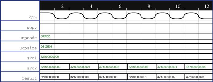
In addition to replicating applicable waveforms from the specification, we should plan on cover points to execute arithmetic operations, and see how the design responds for a predefined set of inputs. So our initial cover point plan might look like this:
• Create cover points that replicate each waveform in the specification that illustrates arithmetic unit behavior.
• Cover each arithmetic operation (ADD, SUB, CMP) with nonzero inputs, alone and back-to-back with another arbitrary operation.
• Cover cases of each operation above with specific data that exercises all bits.
Assumptions
Next we need to consider assumptions. In bug hunting mode, we want to target specific behaviors of the design, which would mean that we might be applying constraints so that behaviors are restricted to checking operations of the choice. We should not shy away from overconstraining while trying to verify specific behaviors. Remember that we might not be able to come up with the right assumptions in the first attempt, and hence we might be spending some time wiggling to converge on all needed assumptions. This is a common practice for any model bring-up. In our case, the initial assumptions for our planned overconstraints on the environment would include:
We should also examine the interfaces we have identified in our block diagram: we will need to make sure our assumption set properly models the behaviors of each of these interfaces. In the case of our simple ALU, we have identified the Instruction Driver Interface and Data Transfer Interface as the points of interaction between our model and the outside world. For this simple example, these interfaces do not have any complex protocol requirements to model with assumptions.
In more complex cases, the interfaces from the design under consideration might align to a standard protocol specification, such as USB, AXI, or AHB, or match a block from a previous design or version. Thus, you may have a set of reusable assumptions (and assertions) that define a protocol, or be able to leverage a similar interface assumption set from a previous project. Be sure to take advantage of any reuse opportunities. In our simple ALU example, we do not have such a case.
If the interfaces are complex to describe in terms of standalone assertions, and we do not have reusable collateral, we might also consider developing reference models, as discussed in the next subsection.
Assertions
Apart from cover points and assumptions, we obviously need to define one more type of property: our assertions, or proof targets. As discussed above, these should largely be inspired by the specification document, which is the official definition of what we are supposed to be validating.
Here are the types of assertions we generate for this example:
• Assert that when a valid operation arrives, a valid output appears in three cycles.
• Assert that each operation generates the expected results: if we select ADD, the output should match the sum of the inputs, and so forth.
Note that both the properties above are end-to-end properties based on the specification: they talk about desired outputs in terms of expected inputs. In more complex designs, you may want to supplement these with whitebox assertions that check intermediate activity on internal nodes. While it is often the case that you can fully describe your specification with end-to-end properties, these will also be likely in many cases to be the most logically complex, encompassing large amounts of logic to prove and challenging the formal engines. We should keep this in mind and think about also creating more local assertions on internal modules and verifying intermediate steps of our computation if we run into complexity issues. We still want to specify the end-to-end properties, but having these smaller properties available during wiggling may significantly improve the efficiency of the debug process.
In addition, as we look at the above assertions, it might appear that they are a bit challenging to write as a bunch of standalone properties. Therefore, this might be a good point to start thinking about reference models.
Reference modeling and properties
So far we have described the property planning in terms of simple standalone cover points, assumptions, and assertions. But depending on the logic that is being validated, the DUT may have a varying degree of complex interaction with the neighboring logic. We often handle this by creating SystemVerilog modules that mimic the behavior of the surrounding logic, and generate the expected results at any given time step. These kinds of modules are known as reference models.
So when should we create a reference model and when would a simpler collection of SVA assumptions or assertions be sufficient?
For assumptions, the creation of an abstraction of the surrounding logic should be guided by the failure scenarios exposed during the verification process. This is because it is almost impossible to know in advance the set of constraints sufficient for a given DUT. The constraints that are necessary depend not only on the interaction between the DUT and surrounding logic, but also on the specifications that are being validated. If adding constraints to the model requires lots of bookkeeping, it is best to develop a reference model that captures this abstraction in a very simple way. In situations that do not require lot of bookkeeping and information tracking from past events, a collection of simple SVA assumptions is usually sufficient. Often it is hard to be sure from the beginning whether you need to represent the full complexity of the neighboring unit in constraints for correct behavior, or if a small set of basic assumptions will suffice. Thus, we usually recommend starting with simple assumptions, which can evolve into an abstracted reference model of the surrounding logic at later stages if required.
However, we should think about potential reference models we might need, and plan for them as necessary. If you have some interface that follows a complex protocol, you are likely to need a reference model. Looking at our specification, we see that in this case there are not many requirements on the inputs. But if our interfaces were more complex, we might look at the Instruction Driver Interface and the Result Transfer Interface and consider what it would take to create reference models.
In addition to environmental reference models for assumptions, we should also think about the possible need for functional reference models for assertions. This is often a solid way to verify complete operation. In general, the RTL implementation of the design would need to take into consideration the timing requirements, debug-related hooks, clock gating, and other requirements. The reference model to be written for FPV can be abstracted to some degree: we need not consider any such requirements and can concentrate just on the functional aspect of the design. We refer to such partial or abstract models of the logic as shadow modeling. These partial shadow models are in general very helpful for the bug hunting FPV and can later be expanded to a complete abstraction model if full proof FPV is needed. A simple assertion that the RTL output will always be equal to the abstract model output would then give you a sense of formal completeness, for the portion of the logic that we model.
Again, in this case we have a relatively simple model, but you can easily envision cases where we are carrying out a multistep arithmetic operation that would be messy to specify in assertions. In this case, we might want to think about modeling the behavior of our ALU operations independently, and just compare the expected results to those from our real model. So we might add to our verification plan:
Addressing Complexity
As part of our FPV plan, we should consider possible actions to reduce the size or complexity of the design, and make it more amenable to FV. This may or may not be necessary, but based on initial size or difficulties in convergence of some properties in our FPV design exercise environment, we should make an early judgment on whether some complexity issues might need to be addressed in the initial FPV plan. We also need to keep in mind the possibility that our initial assertions might prove quickly, but as we add more complex assertions or relax some overconstraints to expand the verification scope, we might need to address the complexity. In Chapter 10 we discuss advanced complexity techniques you can use on challenging blocks when issues are observed during verification, but here we discuss a few basic techniques you should be thinking about at the FPV planning stages.
Staging plan
You should always be careful about trying to verify the fully general logic of your unit from the beginning: while it might seem elegant to try to verify all the logic in one shot, in many cases it will make your FPV process much more complex for the tools, in addition to making debug more difficult. We encourage you to start with an overconstrained environment, focusing on the most risky areas or operations identified in the design.
To maximize the value of our verification environment, we should have a solid staging plan in place to relax the constraints step by step, gradually building our bug hunting FPV into a full proof run. So first we might restrict our verification to one particular data size, DSIZE08, by adding an assumption that the data size has a constant value. Once this restricted environment is stable and debugged, we can relax this condition and try to achieve the same level of confidence as before with more possibilities enabled.
As previously discussed, we also want to ignore the Design For Testability (DFT) functionality and the logic submodule in our initial verification. If we succeed in verifying the arithmetic subunit, our main area of focus, with all data sizes, we optionally might want to consider adding these additional functions back in to the model.
Blackboxes
In addition to considering overconstraints, we should also think about submodules that are good candidates for blackboxing, which means they would be ignored for FPV purposes. We should refer again to our block diagram here, where we have identified the sizes of each major submodule and marked likely candidates for blackboxing. In general, if your block contains large embedded queues or memories, these are prime candidates for blackboxing, though we do not have such elements in the case of our ALU.
When choosing blackboxes, we need to be careful to think about the data flow through our block and what the effects of a blackbox might be. Since we are initially focusing on arithmetic operations, our first identified blackbox, the logic unit, is mostly harmless: the operations we focus on will not utilize this unit. So we will plan on blackboxing this initially, to help minimize the complexity.
However, remember that the outputs of a blackbox become free variables—they can take on any value at any time, just like an input, so they might require new assumptions. For our ALU, we need to add a new assumption when blackboxing the logic unit, so it does not appear to be producing valid logic results for the final MUX:
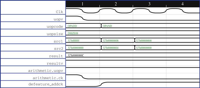
We also identified a secondary potential blackbox target: the decoding block at the front end of the arithmetic subunit. If we have a formal design exercise environment up already (which we recommend as the starting point of an FPV effort, as discussed earlier), it might be useful to bring up a few cover points with the additional blackbox active, and sanity-check the waveforms generated in our FPV tool to get an idea of the additional assumptions that might be required. Such an example is shown in Figure 6.5 below.
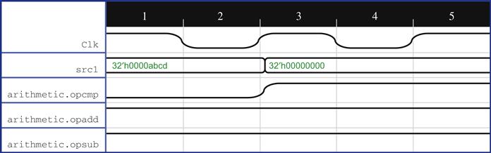
What do we observe now? A few cycles after the start of our waveform, we see a case where all the arithmetic operations are enabled at the same time. This is an unwanted situation and there is no guarantee of any correct result at the output of the block. If you analyze the situation now, we have cut out the block that sanitizes the opcode and generates one and only one operation for a clock cycle. Now all the outputs of the decoder block are free to choose any values and hence we observe something that looks like an insane behavior. We would need to rectify this situation by adding some new assumptions related to the blackbox, or back off and conclude that the decoder is not a good blackbox candidate. Hence, we need to be extra cautious in choosing the blocks in the design we want to blackbox. Since we already determined that this blackbox is not truly necessary, we are probably better off keeping this logic in the model for now.
Essentially, this problem stemmed from the fact that our blackbox candidate was directly in the path of the operations we are checking; we can see that this is much more likely to require some more complex additional assumptions if we blackbox it. In addition, right now our total state count in the un-blackboxed portion of the ALU is comfortably below our target range (40,000 state elements), so we can avoid this additional blackbox unless it is needed. Thus we should initially plan on not blackboxing this subunit, though we can still keep that in mind as a possibility in case we hit complexity issues.
Structural abstraction
Another useful complexity reduction technique is data/structural abstraction, where the size of logical structures is reduced: for example, by reducing the number of buffer entries or restricting the width of a data bus. Structural abstraction not only reduces the size of the logic, and hence the state space, that the tool has to search; it also allows the tool to reach interesting microarchitecture points in the flow at much lower bounds. For example, if there are several corner cases in the microarchitectural flows when a buffer/queue is full, then reducing the size of the buffers from 40 to 4 will allow the tool to explore behaviors around “queue full” at a much lower bound.
These data/structural abstractions are usually very simple and can be fully automated. It is a good idea to work with the RTL designers to parameterize the sizes of various buffers and arrays. The reduced sizes of the buffers should be nested in an ifdef block in the RTL that could be enabled only for FPV. This will allow the FPV user to take advantage of the parameterized values to work with an abstracted RTL model.
For our ALU example, we are in good shape because we have MAXDSIZE as a parameter. Perhaps the mode with an 8-bit maximum size is not really something required in our final product, but having it there lets us do our initial verification in a simpler, smaller environment that is likely to reveal the vast majority of potential bugs.
Quality Checks and Exit Criteria
A passing proof does not necessarily mean that the DUT satisfies the property under all possible input scenarios. Proof development is prone to human errors: it involves the process of debugging failures, adding constraints and modeling to the proof environment, and guiding the process toward the final validation goal. It is crucial that we have quality checks in place to catch these errors or proof limitations as quickly as possible. The major factors that must be considered to judge FPV quality include:
• Quality of the property set being proven: Does the set of assertions provide a good representation of the targeted specification, and exercise all relevant parts of the model?
• Quality of the constraints: Assumptions, blackboxes, and other tool directives are limiting the proof space. Are we sure that we are not ignoring critical behaviors and hiding bugs?
• Quality of the verification: Did the FPV tool achieve a full proof, or a bounded proof at a depth that ensures high quality?
The first fundamental component of FPV quality depends on actually targeting the important aspects of your design. You should make sure that you review your assertions, assumptions, and cover points with architects and design experts. This review should check that you have assertions and cover points for each major piece of functionality you are trying to verify, and that your assumptions are reasonable or correspond to intentional limitations of your FPV environment. If using FPV as a complement to simulation, you should focus on the risk areas not covered by your simulation plan and make sure these are covered in your FPV plan.
Another major goal of quality checks is to make sure that you do not have any proofs passing vacuously, or due to having assumptions and other tool constraints that are so strong they rule out normal design behaviors or deactivate important parts of your RTL model.
As we have discussed in previous chapters, the best way to gain confidence in coverage and prevent vacuity is a good set of cover points. There is a common statement among the FPV experts: “Tell me the cover points and not the assertions to check if your FPV activity is complete.” Most tools auto-generate a trigger condition cover point for any assertion or assumption in the form A |-> B, to check that the triggering condition A is possible. These auto-generated precondition covers are useful, but make sure you do not fully depend on them: good manually written cover points that capture a designer’s or validator’s intuition or explicit examples from the specification are much more valuable.
Another simple test that we recommend for projects with little previous FPV experience is to insert some known bugs (based on escapes from similar designs) and try to reproduce them as part of the process of confirming nonvacuity of your proof environment. This can be especially effective in convincing your management that your environment really is contributing to the validation effort, which can often be an area of doubt if they are primarily seeing reports of successful proofs.
The third major aspect of verification quality is the strength of the verification itself. In the ideal case, your FPV tool will give you full proofs of your assertions, which give you confidence that no possible execution of any length could violate them. However, in practice, you will be likely to have many assertions that are only able to get bounded proofs. In general, this is perfectly acceptable and, in fact, many Intel projects complete their FPV goals using primarily bounded rather than full proofs. Remember that a bounded proof is still a very powerful result, showing that your assertion cannot fail in any possible system execution up to that number of cycles after reset, in effect equivalent to running an exponential number of simulation tests. The main challenge here is that you need to be careful that you have good proof bounds that do not hide important model behaviors.
Checking that your cover points are passing, with trace lengths less than the proof bound of your assertions, is your most important quality check. Conceptually, this shows that the potential executions considered in the proofs include the operation represented by that cover point. Usually it is best to have your assertions proven to a depth of at least twice the length of your longest cover point trace to gain confidence that your proofs encompass issues caused by multiple consecutive operations in your design.
Reconciling your assertions and assumptions with simulation results is another important quality check if you have a simulation environment available that contains the unit under test. Some tools allow you to store a collection of simulation traces in a repository and check any new assumption added against the collection of the simulation traces. This will give early feedback on whether the assumption being added is correct. This should be followed by a more exhaustive check of all the assumptions against a much larger collection of simulation tests as part of your regular regressions. Remember that SVA assumptions are treated the same way as assertions in dynamic simulation: an error is flagged if any set of test values violates its condition. Make sure that these properties are triggered in the simulation runs, which can be reported for SVA by most modern simulation tools. Think carefully about your overconstraints though: some subset of your assertions and assumptions may not make sense in simulation. For example, since we assumed that the DFT functionality is turned off, we need to make sure to choose a subset of simulation tests that do not exercise these features.
We also should mention here that many commercial FPV tools offer automatic coverage functionality, where they can help you figure out how well your set of formal assertions is covering your RTL code. The more advanced tools offer features such as expression coverage or toggle coverage, to do more fine-grained measurement of possible gaps in your FPV testing. Naturally, we encourage you to make use of such tools when available, since they can provide good hints about major gaps in your FPV environment. However, do not rely solely on such tools: no amount of automated checking can substitute for the human intuition of creating cover points that represent your actual design and validation intent.
Exit criteria
We started with defining our goals of the FPV, followed by wiggling the design and exploring it, created a verification plan aligning to the end goal, defined the properties to hit our goal, formulated the staging plan, and understood the abstractions to be done. Now we need to define the exit criteria to confidently exit out of the activity on the design. In order to enable these exit criteria, we suggest you try to continuously measure the forms of quality we describe above, tracking the progress on each of the quality metrics, as well as tracking your proportion of properties passing, and your progress in your staging plan. Assuming you are continually measuring your quality, some natural examples of reasonable exit criteria could be:
• Time Limit: Define a time suitable to exit out of the exercise. While it is common to spend a week on design exercise, we would suggest you spend at least two to three weeks on bug hunting FPV, depending on the complexity of the block considered. When you start seeing more value from the bug hunting mode, exposing new bugs or getting more confidence on some corner cases, you should definitely consider full proof FPV for the block. If moving to full proof mode, you should probably expect at least a doubling of the long-term effort. This will likely pay for itself, of course, if full proof FPV enables you to reduce or eliminate unit-level simulation efforts.
• Quality: We can define our exit criteria based on progress in the quality categories defined above. We may have to modify these quality checks for the current stage in our staging plan: each stage will have some subset of known limitations in our verification quality. If our aim is bug hunting and we have a complementary simulation environment, we may not require that we complete all stages, or we may allow some percentage of property completion rather than full completion of the current verification stage. In general, your quality exit criteria may include:
– Quality of the property set being proven: Make sure the validation plan has been fully reviewed, we have created all the assertions and cover points planned, and all of the assertions are passing.
– Quality of the constraints: Make sure all our cover points are passing and no assumptions are failing in simulation regressions.
– Quality of the verification: Make sure all bounded proofs are reaching an acceptable bound, as judged in relation to the cover points. You may also include some criteria related to the automatic coverage reported by your FPV tools, if available.
• Success Trail Off: As with many validation tasks, sometimes you may reach a point of diminishing returns, where you are starting to see less return on your investment after your FPV environment reaches a certain level of maturity. It is common that after a period of initial wiggling to improve assumptions, you will experience several weeks of rapid bug finding, gradually trailing off as the design matures. You may want to set some criterion related to this pattern, such as ending bug hunting FPV when you have a week go by with all proofs passing to the expected bound and no bugs found by new properties.
So for our exit criteria in our bug hunting FPV plan for the ALU, we might choose these:
• We exercise all our specified covers and prove our arithmetic unit assertions for correct ALU functionality to a bound of 50 cycles, under our chosen overconstraint conditions.
– Due to the logical depth of this design, we expect that all covers will be covered in fewer than 25 cycles; if this turns out not to be the case, we need to reevaluate the bound of 50 above.
Putting it all together
The FPV plan for our ALU, based on the various considerations we described in the previous subsections, is illustrated in Table 6.1. This is a bit more involved than the simple design exercise plan in the previous chapter. Don’t let this scare you off—planning is a critical part of any FV effort. As an example, a consulting firm that ran a “72-hour FPV” stunt at a recent conference (see [Sla12]), where they took a unit sight-unseen from a customer and tried to run useful FPV within 72 hours, actually spent the first 12 hours of this very limited time period studying their design and planning their verification approach.
Table 6.1
Running bug hunting FPV
Now that we have come up with a good verification plan, it is time to begin the verification. We will skip discussion of the basics of loading the model into an FPV tool since that has been covered in the previous chapter and because our starting assumption was that you have already developed a design exercise FPV environment for this model. Part of this would include supplying the necessary tool directives for our initial set of complexity compromises, as mentioned in the FPV plan. This will vary depending on your particular FPV tool, but should result in commands something like this in your control file:
# blackbox logic unit
BLACKBOX inst*.logical
# Turn off dft
SET dftslowrd = 0
Now we will walk through some of the more interesting steps of the initial bug hunting verification.
Initial Cover Points
One of our basic sets of cover points was to check that we are covering each arithmetic operation.
generate for (j= OPADD; j<= OPCMP; j++) begin: g1
arithmetic1: cover property
(( uopcode == j) ##3 (resultv != 0) );
end
endgenerate
Covering these properties would make sure that all the opcodes can potentially be used in our environment. Proving these cover points and reviewing the waveforms would confirm the fact. Let’s assume that our initial covers on these are successful, and we have examined the waveforms.
Next we want to verify a cover point so that, for one particular set of data, the design returns an expected value. We will choose one nontrivial value for an opcode and data and check if the design is behaving sanely. We don’t intend to ultimately specify all the values for each operation, since that would defeat the basic claim of formal that you wouldn’t need to provide any vectors. But these basic covers are written to give a basic understanding of the design correctness rather than complete coverage.
add08: cover property ( ( uopv &
uopcode == OPADD &
uopsize == DSIZE08
) ##1
( src1 == 32'h8 &
src2 == 32'h4
) ##2
result == 32'hC);
The specification enforces that the operation should be initiated one clock cycle before the actual data is applied and the result computation takes two cycles after the data is read in. Execution of this cover will expose us to the basic correctness of the design, and now we are poised to explore much further.
As discussed earlier, we are starting on a piece of RTL that is in the middle of verification churn and we don’t expect very basic bugs. This is just the first set of covers to see if our environment is set up correctly and we can take it ahead. We will probably want to add more cover points, inspired by additional interesting cases we observe while debugging FPV waveforms, as we advance further in our bug hunting.
Extended Wiggling
The process of wiggling is discussed in detail in Chapter 5. We can expect around 10–20 wiggles on a typical unit before we start seeing useful behaviors. It might take even more for complex units. For the simple unit considered in this chapter, we might reach a sane state much earlier in the wiggling cycle. Chances are that we have gone through some wiggling already if we have previously completed FPV design exercise on this unit, so we should not be starting totally from scratch.
We shall begin with the wiggling process on our simple ALU. Just to reiterate, cover points are of paramount importance rather than assertions during the initial stages of FPV. We want to ensure that the basic flows and behaviors we observe in the waveforms are in line with the expectations. One more repetition of this tip is provided here so that we don’t miss the importance of this fact.
We shall not make the common mistake of first starting to prove the assertions, as we already know that covers are much more important at the start of wiggling, and not a secondary consideration. We start by trying to prove the basic cover points we described above, checking that each operation is possible and that a sample ADD operation works correctly on one specific set of values (Table 6.2).
Table 6.2
Initial Cover Point Results on ALU
| Property | Status |
| alu0.g1[OPADD].arithmetic1 | Cover: 8 cycles |
| alu0.g1[OPSUB].arithmetic1 | Cover: 8 cycles |
| alu0.g1[OPCMP].arithmetic1 | Not covered |
| alu0.add08 | Cover: 8 cycles |
Now one of the arithmetic operations is not covered. This is a bit surprising, as we expect all operations to yield correct results in three clock cycles. Remember that an uncovered cover point indicates that some design behavior cannot be reproduced under our current proof setup and assumptions. This means that the failed cover point does not generate a waveform, so debugging it can be a bit tricky. There are several methods we can use to get observable waveforms that might give us a hint about why a cover failed:
• Look at the waveform of a related but slightly different cover point to look for unexpected or incorrect model behaviors.
• Create a partial cover point that checks a weaker condition than the original cover point.
• If the cover point involves several events happening in an SVA sequence, remove some of the events and observe the resulting simpler cover point.
In this case, the failing cover point is relatively simple, so it makes the most sense to use the first method above to bring up the waveform for an already covered cover point and look for unexpected or incorrect model behaviors. Bringing up the waveform for the OPADD operation, we are surprised to see a wrong condition being covered here, as shown in Figure 6.6.
As you have probably observed, this is not correct. We expect the output to become 0x0C for the source inputs of 0x8 and 0x4, after three clock cycles. Here, we see that the result value has been always 0x0C since reset, and hence the cover passes. When we debug further, the reason for the result value being constant is that the state element for the result is not resettable—the flop output can come out with any value. In other words, formal analysis has discovered a rare corner-case scenario, where a nonreset flop gets lucky and randomly achieves desired values.
We also observe that the valid bit for the result is also high throughout and the clock for the flop element is completely gated. We bring in the equation for the clock signal and see that a “defeature bit” signal for the design, which we had not been thinking about as an issue initially, is being driven high after a certain time. Typically, we might speak to the block designer or architect to find out what this defeature bit means: in this case, let’s assume they tell us that this bit will be driven to zero in most real-life usages, so the validation team can safely deprioritize cases where this bit is 1.
Now, we need to fix these two issues:
Once we complete these modifications to our environment and rerun, we should see a real pass, where the cover waveform truly represents the activity we expect. We may also want to amend our FPV plan to document the fact that we added a new overconstraint. But alas, a new failure for the same cover point forces a second round of wiggling to analyze the failure. Repeating the process of observing the waveform for a different but related cover point, we get the waveform shown in Figure 6.7.
We now see that an add operation is taking more than the two clock cycles we expected: it is precisely taking one more clock cycle. This is a definite bug in the design and needs to be fixed. Once we fix the design and rerun, all the cover points pass. After observing the waveforms for each of the passing cover points, and paying especially close attention to the one that had previously been failing, we can convince ourselves that the design is behaving reasonably for our set of cover points.
Now, we turn our attention to the assertions. While we could write a set of standalone assertions checking each operation, this seems like a case where it might make more sense to create a reference model instead, calculating the expected result for each operation. There is a level of abstraction we can apply here, making this more of a shadow model than a full behavioral model: we want to calculate the core results of the logic, without including any of the complexities of a real design such as pipelining, scan, or debug logic. We can also take advantage of overconstraint decisions we made for the initial bug hunting, such as our choice to initially focus on DSIZE 08. In this case, we might initially generate something like this:
module my_arithmetic ( Clk, uopv, uopcode, uopsize, src1, src2, resultv, result );
input Clk;
input node uopv;
input node [3:0] uopcode;
input node [2:0] uopsize;
input node [31:0] src1;
input node [31:0] src2;
output node resultv;
output node [31:0] result;
always_comb isuop = (uopcode == OPADD | uopcode == OPSUB | uopcode == OPCMP );
always_comb begin
opadd = ( uopcode == OPADD );
opsub = ( uopcode == OPSUB );
opcmp = ( uopcode == OPCMP );
end
always_comb begin
unique casex ( 1'b1 )
opadd : result0 = src1 + src2;
opsub : result0 = src1 - src2;
opcmp : result0 = (src1 > src2);
endcase
end;
`MSFF( result1, result0, Clk );
`MSFF( result2, result1, Clk );
`MSFF( result, result2, Clk );
endmodule // my_arithmetic
Once the above module is instantiated or bound inside our main ALU, we can add the following assertion to check that the result in the real RTL matches our reference model:
assert_equi_check: assert property (uopv |-> ##3 (result == my_arithmetic.result ) );
We have written here a very simple model for operations. A simple assertion that the two units should generate the same outputs would cover all possible input combinations and, even more important, give complete coverage of the whole data space for these operations (under our known assumptions and overconstraints). This reference model only covers a subset of operations and data sizes, but is correct for the parts that it covers, assuming the corresponding RTL model is properly constrained to not use other parts of the logic.
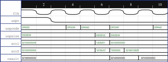
Now that we have written our reference model and are satisfied with the waveforms on our initial coverage points, it is time to try the proofs. When we run with this setup, we see another failure, shown in Figure 6.8.
When we reanalyze the failure, we see that the data on src1 is not being used for the computation, but instead dftdata is used. This comes in because we haven’t disabled the DFT (scan) functionality correctly, despite having planned to do this as one of our initial overconstraints. DFT signals are generally debug-related signals that feed in some sort of pattern through a separate port and help in debug of the existing design, so when running FPV without DFT turned off, it is common to observe cases where the tool figures out clever ways to use it to generate bad results for an assertion. We stated above that we used an overconstraining assumption to set signal dftslowrd to 0, but as we figure out after examining the waveform, this is an active-low signal, and we really need to set it to 1. Once we add the correct DFT constraints, and complete several more rounds of wiggling to work out details that need to be fixed in the assumptions, we get to a point where we have the assertion assert_equi_check passing. Because this is a comprehensive assertion that covers many operations, we should also be sure to review our cover point traces again after the assertion is passing.
Having completed our initial goals in the verification plan, we can consider improving our verification coverage by relaxing some of the initial compromises we made earlier.
A good start would be to relax the constraint that disabled the defeature bit, a last-minute constraint we added based on issues discovered during debug. Since this was a late compromise rather than part of our initial FPV plan, it would be good to find a way to account for it and properly verify its functionality. Instead of driving it to 0, now we should remove this overconstraint and allow it to assume arbitrary values of 0 or 1. This will require figuring out what the expected behavior is for the model under various values of this signal, and refining our reference model to take this new functionality into account.
If that goes well, we then can target the items mentioned in our complexity staging plan to further expand the scope of our verification: allowing all DSIZE values, allowing DFT functionality, and un-blackboxing the logic submodule. Each of these changes will likely require expanding our reference model (or adding a second, parallel reference model) to include these new aspects of the behavior.
As you have probably figured out by now, this is a relatively simple example overall for FPV. This example is taken to show the power of modeling the code and use it for verification. For most real-life units, the wiggling would take many more iterations to reach a stage of useful verification. Don’t be afraid of having to go through 20 “wiggles” to get useful behaviors!
By now, we have good confidence in the environment and the ability to check for various operations.
Expanding the Cover Points
After completing each major stage of our FPV effort, we need to take another look to make sure that we are able to reach various interesting microarchitectural conditions and we are not restricting the model unnecessarily. The initial set of cover points helped us in assessing the quality of the environment we started with and understanding more of the design. The final cover points, inspired by a combination of our knowledge of the specification and our experience debugging the interesting corner cases found during the FPV effort, give us the required confidence that we have not left any stone unturned during our exercise. The cover points are our primary indication of the quality of the verification performed.
Covers at this point of the design are mostly “whitebox.” We should not hesitate to observe internal transitions and known critical conditions of the internal logic. At a minimum, you should be able to translate most of your simulation coverage specifications into SVA cover points and verify. There might be some areas of the design that remain uncovered because we ruled them out through the assumptions. Hence, these covers are very important in assessing the extent of our journey in achieving our FPV goals.
Remember that when relaxing overconstraints and expanding our verification space, we should review our basic cover points once more, since any relaxation of constraints could result in major changes to overall functionality. Chances are some of our basic operations might be covered in different ways, or the cover points might become less useful. For example, when we turn on DFT logic, which allows arbitrary values to be scanned in for each major state element, we may find that suddenly every cover point is covered by a trivial example where DFT turns on and just happens to scan in the correct value. We will need to carefully modify the cover points so they still are truly covering the intended functionality.
Removing Simplifications and Exploring More Behaviors
Let’s assume we have reached the point where we are confident in the verification of the arithmetic logic and have now un-blackboxed the logical subunit, at the same time removing our earlier assumption that restricted us to arithmetic operations. We have likely added an assertion that checks that operations always have the proper latency in our top-level model.
Resultv_correct_wrt_uopv: assert property ( uopv |-> ##3 resultv );
When we try to prove the above assertion, we might get the counterexample shown in Figure 6.9.
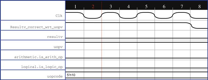
As you can see, there is an opcode 5’h10 that is not defined in the list of acceptable opcodes for the design. Thus, the design behaves erroneously when we try to enable the check for all opcodes in one shot. This is another common situation when relaxing some assumptions and expanding the verification space: allowing a wider variety of legal behaviors has opened the door to a wider variety of illegal behaviors. Thus, we need to add another assumption:
Legal_opcode: assume property
( valid_arithmetic_op ( uopcode ) ||
valid_logical_op (uopcode) );
The Road to Full Proof FPV
Once you are experienced with running FPV on your models, you can start planning from the beginning for full proof FPV, with bug hunting as the initial stage of your plan. If you are less experienced, you first want to embark on bug hunting FPV, and may think about expanding to full proof based on the success of these efforts. Could you verify all the requirements of the specification, making simulation-based unit-level verification redundant for your current module?
In the case of our ALU example, it looks like full proof FPV might indeed be a reasonable target. Once we have gone through all the steps identified in our complexity staging plan and found that adding more generality to our proofs did not cause a complexity explosion, we can take a step back and ask the question: can we make this a full proof environment and back off from our simulation effort?
Be careful before making this leap: because our initial plan was based on bug hunting, we have some important questions to ask about the completeness of our verification. When focusing on bug hunting, it was sufficient to come up with a small set of interesting properties, which helped us to find and reveal some set of bugs. In general, we must plan for a greater level of rigor in our quality checks to have confidence in full proof FPV. We need to ask the harder question: do we have a complete set of properties, which fully checks all the requirements of our design specification? Remember, just because your FPV run includes the entire RTL model, or mechanical measures of coverage from your tool claim that all lines are exercised, it does not mean that you have fully verified the specification.
In most cases, your main specification is an informal document written in plain English (or another nonmachine language), so there is no easy way to answer this question directly. You must carefully review this document, and make sure that each requirement listed is translated to an assertion, or can be described as nontranslatable. You also need to check that your assertions are as strong as necessary to fully enforce your specification. For example, suppose instead of our assertion requiring a latency of 3, we had written an assertion like the one below that just said we would eventually get an answer:
resultv_correct_sometime: assert property
(uopv |-> s_eventually(resultv));
This would seem to be checking the correctness of our ALU, and might help us to find some bugs related to completely dropped operations, but actually would be failing to fully check the latency requirement.
Checking assumptions and cover points is also a critical part of this review. You must make sure all major operations are covered by your cover points, in order to ensure that you are not leaving any gaps in the verification. You should also review your assumption set and make sure it is not unexpectedly ruling out analysis of any part of the specification. Once you have done this, be sure to present your proposed set of specification properties to your design architects and get their buy-in that your verification plan truly is complete.
In the case of our ALU, the overall functionality is very well-defined: we have a set of operations, and for each one, we need to make sure it generates proper output based on its inputs. We also need to check for the corner-case exceptions such as DFT, which we excluded from the initial bug hunting FPV, and make sure our unit operates correctly under these circumstances. We should make sure that we create assertions describing correct operation of each of these exceptions, as well as cover points to double-check that each one can be exercised under our final set of assumptions.
Do not let the need for increased rigor scare you away from attempting full proof FPV. As long as you pay close attention to the requirements of your design specification, this is often very feasible at the unit level, and can be a much smaller overall effort than validating through a comprehensive simulation testbench. In any case, the need for careful reviews is not really a new requirement introduced by FPV: the same concerns and hazards, such as the danger of incomplete or overly weak checking, apply to simulation and other validation methods as well. Full proof FPV has been successfully run on selected units on many projects at Intel and has been found to result in significantly higher design quality for lower effort in the long run.
Summary
In this chapter, we have reviewed the typical process of using FPV for bug hunting and full proof mode, using our example of a simple ALU. Bug hunting is the use of FPV as a supplement to other validation methods, to detect hard-to-find corner-case issues. Full proof FPV is the attempt to fully prove your specification, completely replacing other validation methods.
You should start by trying to identify a good target unit for FPV. Try to find a piece of logic that will have under 40,000 state elements, after appropriate blackboxing of large memories and other state space reductions. Then you should look at a block diagram, identifying your primary verification focus areas, marking the sizes of individual subunits, and labeling major interfaces and potential blackbox candidates. Using this information, you should then create an FPV plan, including major goals, important properties, complexity compromises and staging, and a good set of exit criteria.
We walked through this process on our ALU example, showing how we would come up with an initial bug hunting plan, and demonstrating some of the initial steps as we begin to put this plan into action. Naturally a real-life verification effort would likely have many more wiggling steps than we could describe in the text of this chapter, so our goal was just to demonstrate the general idea. Once we showed how the initial steps of this verification might be completed, we went on to discuss how we could expand this to a full proof FPV effort, which could potentially replace simulation-based verification for this unit.
Practical Tips from this Chapter
6.1 For validation-focused FPV, choose blocks that primarily involve control logic or data transport, with data transformation limited to simple operations like integer addition.
6.2 When planning for bug hunting FPV, use overconstraint as needed to simplify the model you work on, in order to focus on your current problem areas.
6.3 When first trying FPV on any new design, start with lightweight design exercise FPV (as described in Chapter 5) to verify basic behaviors and FPV feasibility before moving to more elaborate validation-focused FPV efforts.
6.4 Carefully carve out the logic you want to verify with FPV and limit the design to a size that can be handled by the tools. A good rule of thumb with current-generation tools is to aim for less than 40,000 active state elements (latches and flip-flops).
6.5 When beginning the bug hunting or full proof FPV planning process, start with a block diagram of your unit, including the sizes of all major blocks, and label the interfaces, blackbox candidates, and areas of verification focus. This diagram will provide a critical foundation for your verification plan.
6.6 Create a verification plan when beginning a validation-focused FPV effort. This should describe the logic to be verified, properties and cover points, staging plan, decomposition strategy, and success criteria.
6.7 Explore the opportunity of reusing standard properties whenever applicable to your units: this can save you significant time when bringing up an FPV environment.
6.8 If you start generating a lot of assumptions or assertions with complex interactions, consider creating a reference model and basing the properties on its behavior.
6.9 Start with simple constraints on the inputs and slowly evolve into an abstracted reference model of the surrounding logic, if required.
6.10 Don’t be afraid to model the code from the specification. A simple assertion that the model output is equal to the implementation output is often a solid way of proving a design formally.
6.11 When thinking about blackboxing a submodule, look at waveforms involved in common operations, extracted from simulation or design exercise FPV cover points, to help decide whether you would need complex assumptions to model relevant outputs.
6.12 Structural abstractions not only reduce the size of the logic and the state space, but also allow the tool to reach interesting microarchitectural points at much lower bound.
6.13 Work with your designer early in the design cycle to parameterize the RTL code such that it becomes easy for you to reduce structure sizes during FPV.
6.14 Make sure that you review your assertions, assumptions, and cover points with architects and design experts, as part of the validation planning process. Include FPV in the validation plan, and check that the properties you create are covering the aspects of functionality not being covered by simulation.
6.15 Carefully check that your cover points, including both automatically generated assertion/assumption triggers and manually created covers that represent major design operations, are passing. If not, it means you have a likely vacuity issue.
6.16 If you are using bounded proofs, make sure that your assertions are proven to a depth greater than your longest cover point trace, preferably at least two times that trace length.
6.17 Make sure that you attach the FPV assumptions as checkers in the dynamic simulation environment, if available, so that you can gather feedback about the quality of your formal environment.
6.18 Use automated coverage features of your EDA tools to gain additional feedback about coverage, but do not treat these as a substitute for a good set of human-created cover points based on your design and validation intent.
6.19 Begin any FPV effort by creating a set of reasonable cover points on your model, representing typical and interesting activity.
6.20 Don’t get carried away by initial cover passes. Take an extra step to view and analyze if the intention is truly replicated in the waveforms.
6.21 Remember, just because your FPV run includes the entire RTL model, it does not mean that you have fully verified the specification. You need to check that your assertion set is complete.