
Dealing with complexity
In Chapter 10, we describe ways to address complexity issues, enabling formal verification on designs that initially might seem too large or logically complicated for tools to handle. After reviewing the general concepts of state space and complexity, we describe several complexity reduction techniques on a memory controller example. Simple techniques include black boxing, case splitting, property simplification, and cut points. Generalizing analysis with free variables is also often useful. We then describe several types of abstraction models: datapath abstraction, symmetry exploitation, counter abstraction, sequence abstraction, and memory abstraction. We conclude with descriptions of creating partial “shadow” reference models, and helper assumptions that can sometimes rule out large parts of the problem space. Together these techniques have enabled successful verification of large and complex models; do not give up on formally verifying a model until you have closely examined it for these kinds of opportunities.
Keywords
complexity; NP-completeness; state space; abstraction; simplification; free variables; cut points; symmetry
Designs are tuned to the extent that they are almost wrong.
—Roope Kaivola
Formal verification (FV) engines have made amazing progress over the past three decades, in terms of the sizes and types of models they can handle. As we have seen in the previous chapters, FV can now be used to address a wide variety of problems, ranging from targeted validation at the unit level to solving certain types of connectivity or control register problems on a full-chip design. But we still need to remember one of the basic limitations we described back in Chapter 1: FV tools are inherently solving NP-complete (or harder) problems, so we constantly need to think about potential compromises and tricks to handle complexity.
How will you know if you are facing complexity issues in your FV tasks? The complexity problem can manifest itself as memory blowups, where memory consumption increases until your machine capacity is exhausted, or as cases where some proofs never complete. You may also see a tool crash or timeout related to these causes. Solving complexity in the FV domain requires some clever techniques, very different from the solutions deployed in simulation.
In this chapter, we start by discussing state space and how it is related to design complexity. We then move on to some more detailed discussion of some of the techniques discussed in our earlier chapters, such as blackboxing, cut points, driving constants, and decomposing properties. Then we introduce some fancier techniques that can result in significant increases to the capabilities of your FV runs.
In this chapter, we focus on an example using formal property verification (FPV), but most of the general principles we describe will apply to other forms of FV as well. Whether you are hitting complexity issues in FPV, formal equivalence verification (FEV), or one of the more specific FPV-based flows, you should think about how each of these methods might apply to your design.
Design State and Associated Complexity
The design state consists of the values of each input and state element at a particular moment in time. The state elements include flops, latches, and memory elements. If we consider a simple design with n state elements, theoretically, we would have 2n possible configurations. These state elements in conjunction with the number of inputs (m) and their combinations (2m) would form the full design state that could be conceived. The total number of such conceivable states for a design would be 2(n+m). Simple math would reveal that the number of possible states in a trivial design with 10 inputs and 10 flip-flops to be 220, or 1,048,576. We can now imagine the number of states that would be possible for realistic designs and the number needed to analyze state changes over time. Given this inherently huge state space, it is somewhat amazing that with current EDA tools, we can often run FV on designs with around 40,000 flops, analyzing behavior spanning hundreds or thousands of time steps, and not experience noticeable complexity issues.
As we have seen in the discussions in earlier chapters, after reset, a design will be in one of the states, termed “reset state” of the design. Normally, only a small subset of the state elements is initialized by reset, with the rest left unconstrained and treated by FV tools as if they could assume any arbitrary value, as long as it does not violate any assumptions. Thus, the number of possible valid reset states is generally more than one and they form a small region in the state space rather than a single unique state. FV effectively analyzes all reset states in parallel.
The real-life operation or simulation of a register transfer level (RTL) design can be seen as a meandering path through the state space starting at reset. As a design operates, it transitions from a reset state to other states at each subsequent clock tick. Thus, it traverses one point in the state space to another, forming a trajectory. Simulation or emulation tools examine one trajectory at a time, while formal tools analyze all such trajectories in parallel. This concept can be well understood by the state space diagram in Figure 10.1.
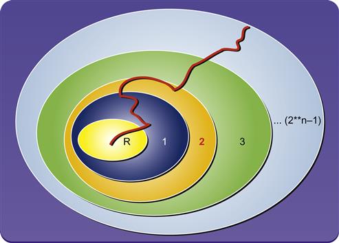
As can be observed from the diagram in Figure 10.1, the design starts with the reset state (the oval labeled R). The possible states during the first cycle are depicted by oval {1}. Similarly, states possible in the second cycle are shown by oval {2}, and so on. The design would start its traversal from the {R} state and work through the next set of states until it reaches the final state. A typical simulation test would explore one trajectory at a time as depicted in the illustration. FV would explore all states possible in each clock cycle, as represented by the growing series of ellipses in the diagram.
If the FV tool reaches a full proof, it has effectively explored all these ellipses out to include all possible states reachable by the design. If it does a bounded proof, it is still covering a very large region of the space in comparison to simulation; the outer circle in Figure 10.1 represents a proof to a bound indicated by the outermost ellipse, which represents some specific number of cycles. It would guarantee that there is no failure possible within that bound, but the design might fail outside that range. All the regions in the diagram are not equal, due to varying complexity of the logic: small increments in the depth achieved can be hugely significant depending on the property being checked. For example, a design may spend 256 cycles waiting for a startup counter to complete, and then start a very complex operation when the count is done. In that case, analyzing each of those first 256 cycles may be easy, while the cycle after the counter completes may expose the full logic of the design.
This exponentially growing state space is a major source of complexity issues for FV. This difficulty, known as state space explosion, is a typical culprit preventing us from achieving the full convergence on the design.
We should point out, however, that the above discussion pertains to types of FV that analyze behavior over time: FPV, or sequential FEV. Combinational FEV, since it breaks up models at state elements, allows a much simpler analysis by formal tools: they just need to comprehend the Boolean logic that describes the next state at each latch, flop, and output for a single cycle. But remember that even analyzing correctness of a single state is an NP-complete problem (equivalent to the SAT problem), so it is possible that complicated RTL logic can cause a complexity blowup even in combinational FEV. Although the focus of this chapter is on the more difficult complexity problems encountered in sequential FV techniques, many of the methods described in this chapter can be useful with combinational FEV as well.
Example for this Chapter: Memory Controller
To make the examples in the chapter more concrete, we will consider a memory controller interface, with the basic structure shown in Figure 10.2.
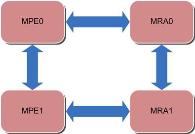
The block here contains two memory protocol engines (MPEs) and two memory read/write arbiters (MRA). The protocol engines and the arbiters are tightly connected to each other to work in tandem to access the memory locations from various memory modules and serve a range of requestors.
The memory arbiter selects between several requestors vying to send a memory address and request using the following priority scheme:
Refresh > Read > Write
One other important function of the MRA is to check and avoid hazards like read after write (RAW), where a read in the pipeline may return a value that predates a recent write. This hazard check requires an address compare operation. The controller is a fully contained block that makes sure the memory access functions are hazard free and guarantees correct data storage and retrieval.
The MPEs contain a wide variety of decision finite-state machines (FSMs) and implement a multitude of deep queues to store the in-flight content and perform some on-the-fly operations. The MPEs enforce protocol adherence and maintain many data structures to ensure consistency.
Some of the properties that are hard to converge for this controller are:
• Fair arbitration across all read and write requests
• Faithful data transfer through the controller
• Priority preserved across all requestors
In the remainder of this chapter, we will often refer to this example as we discuss how we might use various techniques to handle potential complexity issues during its FV.
Observing Complexity Issues
Complexity issues in FV manifest themselves as:
• Memory blowups—Caused by the state explosion problem and resulting in insufficient resources. Sometimes it also results in system crashing or angry emails from your network administrator.
• Indefinite runtime –While the tool works on the problem within a defined set of resources, it is continually exploring more states and never completes within a stipulated time period.
• A low bound on the bounded proof—Bounded proofs are often okay if the bounds are reasonable, but a low bound that fails to match cover point requirements or that fails to exercise interesting logic is not acceptable.
• Tool crashes—When system capacity is stressed for any of the above reasons, tools sometimes fail to report this cleanly and crash instead.
As you saw in Chapter 6, we advise that you begin FV efforts with an attempt to estimate complexity issues in advance, by planning your verification with the aid of a block diagram and your knowledge of major submodules. The design itself could be too huge to be handled by typical FV tools, and you may need to focus on lower levels or find major blackboxing opportunities. The design might also contain many memory elements that are wide and deep, a large set of counters, or logic styles (such as floating point arithmetic) that do not cooperate well with your tool set.
The first general estimate can be obtained from the number of flops in the module that is under test. A finer estimate would be to assess the number of flops in the logic cone of each assertion; this information can often be reported by your FPV tools. A number of flops might also be added to the cone of logic for proving the assertion because of the constraints that are coded. As we have mentioned, a rule of thumb we use is that your tool should not need to analyze more than 40,000 state elements. You can try with more than this and may find that your tools continue to work reasonably well, but as you grow the number of state elements, expect to spend more time dealing with complexity.
Also, do not forget that model-checking engines used in typical FPV tools are getting smarter day by day, which means that even though we suggested a rule of thumb of aiming for less than 40,000 state elements, they can sometimes converge on bigger design sizes (that rule of thumb may be outdated by the time you read this book!). Designs that were deemed not fit for convergence through FV a couple of years ago are easily going through the latest engines. The EDA industry and academia are actively working and collaborating on improving engines. There is somewhat of an arms race going on here though; while the engines further their convergence capabilities, designs also continue to grow in complexity.
As we mentioned in Chapter 6, we also suggest initially targeting bounded proofs rather than full proofs, since these are often much less expensive to obtain. Use your knowledge of the design and a good set of cover points to try to estimate a reasonable bound. Most projects we have worked with at Intel were comfortable with accepting a bounded proof in place of a full proof as a signoff criterion, as long as the bound was well justified. Thus, before making major efforts to deal with complexity, because your proofs are bounded rather than full, be sure to consider whether the bounded proofs are good enough for your current problem.
Simple Techniques for Convergence
Before we start describing more advanced complexity techniques, we should review and expand upon the basic methods that were discussed in earlier chapters. If you do encounter a complexity issue, be sure you attempt to make full use of each of these suggestions.
Choosing the Right Battle
When we choose the design hierarchy level for formal proof development, we need to make sure that we are not biting off more than we can chew. We need to identify the right set of logic where our tools are likely to converge, but where our analysis region is large enough to encompass an interesting set of proofs without requiring massive development of assumptions on the interface.
Let’s look again at our memory controller example. When we look at the number of state elements in the memory interface block as a whole, we might find that the amount of logic is too large, on the order of 100K state elements after blackboxing embedded memories. Thus, we are unlikely to get full convergence on the properties. If this is the case, it might be a good idea to verify the MPE and MRA blocks separately. Because there are two instances of each of these submodules (identical aside from instance names), in effect we would only have to verify 1/4 as much logic in each FPV run, which is a powerful argument in favor of this method. On the negative side, this would create a need for us to write assumptions that model the inter-unit interfaces between the MPEs and MRAs, which we would not have to do if verifying the top-level unit.
We also need to consider the issue of locality of the property logic. Most FPV tools have intelligent engines that try to minimize the amount of logic they are using in each assertion proof, only bringing in the relevant logic affecting that assertion. Even though the full model may have 100K flops, if we expect that each of our assertion proofs will be almost entirely local to one of the MPE or MRA submodules, it may be that we do not pay much of a complexity penalty for loading the full model.
One issue to be cautious of when deciding to run on the lower-level models is that we may initially underestimate the level of assumption writing that needs to be done. If during our initial wiggling stages, where we are looking at counterexamples and developing additional assumptions, we find that our set of assumptions grows too large or unwieldy, we may want to consider backing off our approach of verifying the subunits. We would then verify the full unit, with the logic of all four major submodules combined, and be prepared to look at other techniques for reducing complexity.
Engine Tuning
Before trying any fancier complexity techniques, make sure you are taking full advantage of the engine features offered by your FV tool. Most current-generation FV tools contain multiple engines, implementing different heuristics for solving FV problems. These engines are often tuned to optimize for certain design structures and it is highly recommended that you choose the right set of the engines to solve the problem you are trying to verify. Information about the engines is typically available from the user guide or the data sheets of vendor provided tools. Some engines are good at bug hunting, so are the best choice when you are in early design or validation stages and are expecting many property failures. Others are optimized for safety properties and some at converging liveness properties. Some engines are programmed to function by iteratively adding logic to the analysis region to achieve convergence, while others search deep in the state space to hit hard cover points.
In many cases, individual engines provide certain “knobs,” additional optional parameters for controlling their behavior more directly. Look for the following opportunities for finer-grained control over your engine behavior:
• Start: You may be able to control how deep in the state space the engine should start looking for counterexamples: perhaps you suspect an error when a 64-deep queue is full, for example, so you might tell the engine to start searching at depth 64. This may hurt performance if there was a much shorter failure to find, however. You also have to be careful to check whether this option will cause your engine to assume there are no earlier failures, in which case the proofs may be logically incomplete in cases without a failure. We have also experimented with a “swarm” strategy where a user runs many copies of the FV run in parallel on a pool of machines, each with a different start depth, to try to maximize the speed at which they find the first failure, at the expense of spending significantly more compute resources.
• Step: Similarly, for engines that incrementally move more deeply into the verification space, you might be able to tell them to check for failures every n cycles, for some n, rather than at every possible depth. Again, this is more appropriate when you expect failures, since depending on your tool, it may cause some to potentially be missed, or hurt performance if it causes the engine to skip over easy failures.
• Waypoints: Some engines, also known as “semiformal” engines, try to start by finding interesting individual traces deep in your design space, and then explore the complete space from there. In such engines, specifying a waypoint, or interesting cover point that you think might result in potential failures soon afterwards, can help direct the search. This technique actually can be implemented manually, as we discuss in a later section below, but we mention it here since some FPV tools have lightweight semiformal capabilities built into their engines. Your tool may also contain some nonsemiformal FPV engines that can use waypoint information in clever ways to guide the search process.
Blackboxing
Blackboxing, or marking submodules to be ignored for FV purposes, is one of the major techniques for reducing complexity of a design. When a module is blackboxed, its outputs are treated as primary inputs to the design: they can take on any value at any time, since their logic is not modeled. Because it is relatively easy to do with most tools and can have huge effects on FV performance, you should think about opportunities for blackboxing at the beginning of any FV effort.
One nice aspect of this technique is that it is guaranteed to never create a false positive (aside from the lack of verification of the blackbox itself). This is because blackboxing a module makes its outputs more general: the FV tool may produce additional false negatives, spurious counterexamples that the user must debug and use to suggest new assumptions, but will never report an assertion passing if it is possible that some actions of the blackboxed module could have caused it to fail. Thus, it is safe to blackbox too much logic, and later un-blackbox if too many incorrect counterexamples result.
There are many common types of logic that should almost always be blackboxed for FV purposes, since they either contain styles of logic for which common FV tools are not well suited, or are known to be verified elsewhere. For example, caches and memories are really hard to analyze, due to their gigantic state space, and the functionality of data storage and retrieval is usually not very interesting. There are alternate methods of proving the functional correctness of the memory elements and caches, using specialized formal or simulation tools.
In general, if you see any of these in a unit on which you are planning to run FV tools, strongly consider blackboxing them:
Parameters and Size Reduction
Be sure to look in your model for opportunities to reduce the size of a large data path or large structure. For example, if our MRA contains an N-bit wide data path in which essentially the same logic is used for every bit, do you really need to represent the full width of the data path? Often you can reduce it to a handful of bits, or even a single bit, and still have confidence that your FV proofs ultimately apply to all bits of the bus.
To better enable this method, you should work with your design team to make sure that your RTL is well parameterized. If every submodule of the MRA has a DATA_WIDTH parameter they inherit from the next higher level, making this size reduction in the MRA FPV environment could be a one-line change; but if there are a dozen submodules that each have the N hardcoded to some number, say 32, this edit would be painful.
In other cases, you may have several instances of a block, but be able to essentially run your verification with only a single instance active. In our memory controller, is there significant interaction between the two MPEs, or can the majority of our properties be sensibly proven with one of the two identical MPEs blackboxed, or with a top-level parameter modified so there is only one MPE?
Case-Splitting
When we have large parts of the logic operating separately and we try to verify a very general property, we often end up effectively verifying multiple submachines all at once. This can add a lot of logic to the cone of influence. In our memory controller example, if you have chosen to run your proofs at the top level, do operations tend to exercise all four major submodules (MPEs and MRAs) at the same time, or do different types of accesses essentially exercise subsets of them independently? In the arithmetic logic unit (ALU) example we discussed in Chapter 6, where there are two sets of operations (adder and logic ops) that go to completely different subunits, do we really need to verify all operations at once? Trying to do unnecessarily general property checking that encompasses large portions of the logic all at once can result in significant complexity issues.
You should be sure to examine your design’s care set (set of input conditions you care about-- as opposed to don’t care about-- to verify) and identify opportunities for case-splitting, adding temporary constraints to restrict each proof attempt to a subset of the design logic. This may also create an opportunity to perform independent runs on a network of workstations, so the subproblems can be verified in parallel.
Table 10.1 depicts how the case-splitting might be done on an example care set. Case-splitting would decompose the care set into multiple slices that could be effectively handled by the tools. The cases may be symmetric, or some may encompass more data than others: in the example in Table 10.1, the validator suspects that boundary opcode value 8’h80 will have unique difficulties, so that case has been separated out, while the other cases cover wider ranges. In addition, there may be special modes to handle; the split in this table also has one case for scan mode, in which all opcode values (for that mode) are handled. For each case, you need to add assumptions that set relevant inputs to restricted or constant values, which only exercise the chosen case.
Table 10.1
Example Case-Split of Care Set
| Case | Opcode Range | Scan Mode |
| Case 1 | 8’h00-8’h7f | OFF |
| Case 2 | 8’h80 | OFF |
| Case 3 | 8’h81-8’hff | OFF |
| Case 4 | All | ON |
Be careful, however, to ensure that you have proven that the sum total of all your cases truly covers all possible operations of your design. As we saw in Chapter 9, if you are not careful, you can end up ignoring parts of your design space while splitting up cases. Unlike techniques such as blackboxing, case-splitting can be unsafe and lead to false positives, since you are introducing assumptions that restrict the verification space for each case. If aiming for full proof FPV or FEV, you need to have a strong argument or formal proof that the sum total of your cases covers all activity of your design.
You also need to think about whether the different cases are truly independent, or can interact with each other: think about cross-products. For example, in our memory controller, while we might be able to create independent proofs that individual memory read operations on MRA0 and MRA1 are correct in the absence of external activity, do we need to worry about cases where the two MRAs are acting at once or quickly in succession, and their operations may interfere with each other? If so, after we complete our initial proofs for the split cases, we may still need to run proofs on the full model without case restrictions. This does not mean our case-split was a bad idea however: it is very likely needed to enable us to more quickly find and debug an initial set of issues in bug hunting FPV, even though it leaves some gaps if our goal is full proofs.
One other point you should keep in mind is that sometimes one level of case-splits might not be sufficient, and we might need secondary case-splits to bring complexity under control. For example, if we find that we still have a complexity issue in the ALU from Chapter 6 after restricting the opcode to arithmetic operation, we may need to further split down to create individual proof environments for ADD, SUB, and CMP operations.
Property Simplification
There are numerous cases where you might be able to make your assertions much simpler for the formal tools to analyze, by rewriting them in a simpler form or splitting a complex assertion into multiple smaller assertions.
Boolean simplifications
If you have a property with an OR on the left side of an implication or an AND on the right side, it can easily be split into multiple smaller properties. Of course you can probably come up with other simple transformations, based on principles such as the Boolean laws we discussed in Chapter 2. Smaller and simpler properties are likely to be much better handled by the FPV tools and ease convergence, which also provide significant debug advantages.
The simplest examples of this kind of transformation are replacing
p1: assert property ((a || b) |-> c);
p2: assert property (d |-> (e && f));
with
p1_1: assert property (a |-> c);
p1_2: assert property (b |-> c);
p2_1: assert property (d |-> e);
p2_2: assert property (d |-> f);
If you think about it a little, there are many opportunities for similar transformations of more complex properties, since a sequence may often represent an implicit AND or OR operation. For example, we could replace
p3: assert property (A ##1 B |-> C ##4 D);
with two simple properties
p3_1: assert property (A ##1 B |-> C);
p4_1: assert property (A ##1 B |-> ##4 D);
This technique can be generally applied on protocol assertions like req-ack handshakes. Instead of writing a complete assertion for the whole behavior, we can break down the property into its component elements, based on the arcs of its timing diagram. Be careful, though, that you have a strong logical argument that the sum total of your decomposed properties is equivalent to your original property.
Making liveness properties finite
One other type of property simplification we should discuss relates to liveness properties, assertions that describe behavior that may extend infinitely into the future. These are generally harder for formal tools to fully analyze, so sometimes limiting the unbounded nature of liveness can help in convergence. The new limit defined should have a large enough number to mimic a large bound that it seemingly appears as a liveness condition.
For example,
will_respond: assert property {req |-> s_eventually(rsp)}
might be replaced by
will_respond50: assert property { req |-> ##[1:50] rsp }
Here we are assuming that you have a model with a logical depth significantly smaller than 50, and a good set of cover points showing that a reasonable set of operations of your model could occur within that time limit. Some model-checking engines work much better with a defined bound and could converge faster.
While this technique creates a stronger assertion, and is thus technically safe from false positives, you will often find that it causes a bogus proof failure due to external inputs not responding within the specified time. Thus, when using this technique, you may also need to add companion assumptions that force external readiness conditions to be met within a related time boundary. For example, if in our design there is a backpressure signal that may prevent a response, we would need to make sure that signal changes within 50 cycles:
bp_fair50: assume property (req|->
##[1:50] !backpressure);
Similarly, limiting the bound of potentially infinite-time assumptions is sometimes helpful to verify design properties. For example, the above bp_fair50 assumption might be an appropriate bounded replacement for a more general liveness assumption like:
bp_fair: assume property (req|->
s_eventually(!backpressure));
Putting a finite bound on assumptions, using bp_fair50 rather than bp_fair, is also often helpful in reaching interesting states in the formal analysis. However, keep in mind that such simplifications are technically a form of overconstraint and thus can be potentially dangerous. It is always advisable to constrain the design under test (DUT) as loosely as possible. Removing these delay constraints would give the engines higher freedom to explore deeper state space. If you use these techniques to address convergence issues, we would advise extra review, and consider relaxing them after your initial round of FV is complete.
Cut Points
As we have mentioned in earlier chapters, a cut point is a location in the model where you “cut” a node away from its input logic cone, allowing it to freely take on any value. When a node is cut, the FV tool can then remove the node’s input logic from formal analysis. It is a similar concept to a blackbox: you can think of a blackbox as a case where every output of a submodule has become a cut point. Using cut points is a more fine-grained technique, targeting individual nodes in a design. As we discussed in Chapter 8, the key points used by FEV can also be thought of as a type of cut point.
Like a blackbox, applying a cut point is always a logically safe transformation, possibly introducing false negatives, but never risking a false positive. Cut points increase the space of legal behaviors, since the cut point’s fanin logic is treated as returning a fully general arbitrary value, but often with the benefit of a decrease in the complexity of the remaining logic. If the removed logic truly was irrelevant to the proof, you should see correct results after adding a cut point. If you made a mistake and the logic you removed was relevant, this should be apparent when debugging the false negatives, and you see the cut point value affecting your result. You may need to add related assumptions to model the missing logic, or choose a different cut point.
To see an example of where you might find a good cut point, let’s look again at the memory controller example. You may recall that the MRA arbiter checks for a RAW hazard and performs certain actions as a result. Suppose we trust the logic that computes whether we have a RAW hazard (perhaps it was reused from a previous successful project), and are not worried about verifying that calculation. The intent of the property being checked is to verify that the read is properly delayed when we have a RAW hazard; for the purposes of this check, it does not really matter whether there was a real RAW hazard embedded in the operations performed. Hence, we can safely place a cut point at the output of the RAW computation as depicted in Figure 10.3. The RAW bit is then a free variable and can take any value for the verification.
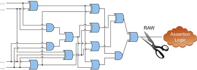
Now the complexity of the logic being checked is drastically reduced, since we are skipping all the logic that computed whether we had a RAW hazard. Since the RAW bit is free to take any value, we might hit false negatives and have to add some assumptions on the bit to make it realistic. For example, maybe the nonsensical case where a RAW hazard is flagged during a nonread operation would cause strange behavior.
If you are having trouble identifying cut points for a difficult property, one method that can be helpful is to generate a variables file. This is a file listing all the RTL signals in the fanin cone of your property. Most FPV tools either have a way to generate this directly, or enable you to easily get this with a script. There may be hundreds of variables, but the key is to look for sets of signal names that suggest that irrelevant parts of the logic are causing your property fanin to appear complex. For example, you may spot large numbers of nodes with “scan” in the name, and this would indicate that one of them is probably a good cut point to remove scan-related logic.
In combinational FEV, you can think of the combinational method as having predefined all state elements as cut points to optimize the comparison. Adding additional non-state cut points for combinational FEV, or adding state or non-state cut points for sequential FEV, can significantly improve performance. Just as in FPV, though, you need to be careful if you are removing critical logic, and may need to compensate by adding assumptions.
We should also mention here that in some cases, we have found that we can successfully run a script to find good FEV cut points through a brute-force method: look for intermediate nodes in the logic of a hard-to-prove key point with similar names or fanin cones in both models, and try to prove the intermediate nodes are equivalent. If the proof succeeds, that node is likely a good cut point. This can be time consuming, but running a script over the weekend that focuses on a particular logic cone of interest can sometimes be successful in finding useful cut points.
Blackboxes with holes
One specific application of cut points that you may sometimes find very useful is the idea of creating a blackbox with “holes”—that is, where a submodule is almost completely blackboxed, but some small portion of the logic is still exposed to the FV engine. This is often needed when some type of interesting global functionality, such as clocking or power, is routed through a module that is otherwise blackboxed for FV. This situation is illustrated in Figure 10.4.
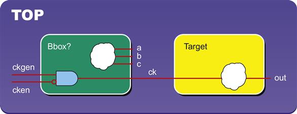
In Figure 10.4, we want to blackbox the block on our left while running FPV at the TOP level, but this causes our proofs to fail in the target block on the right, due to a dependence on some clocking logic that is inside the blackbox. To fix this, instead of declaring the module as a blackbox, we can write a script to add cut points for all outputs of the module except the outputs we want to preserve. In our example, we would want to preserve the input logic for output ck, and the script should find and cut the other module outputs (points a, b, c). Utilizing the script, we effectively create a blackbox with a hole to preserve the one piece of logic we need.
Semiformal Verification
In the section on engine parameters above, we introduced the concept of “semiformal” verification. This is worth more discussion here, because even when your tool has a built-in semiformal engine, understanding details about the underlying method can enable you to use it much more effectively. Suppose you are in a bug hunting FPV environment, and you find that your tool is getting stuck attempting to hit a deep cover point. For example, you might run your tool for a week, getting to bound 1,000 in your proofs, but find that one of your cover points still has not been hit. In our memory controller example, suppose we have a refresh counter that initiates a special action every 213, or 9,192 cycles. It is likely that our tool will never be able to reach such a depth, due to exponential growth of the state space. But we might be very concerned about checking for potential errors that can occur when the refresh condition is hit. Is there any way we can search for such a bug?
A simple solution is to think about semiformal verification. Instead of starting from a true reset state, we will provide an example execution trace to the tool as a starting point. Most FPV tools allow you to import a reset sequence from simulation, so we could just harvest a simulation trace that ran to 9,000 cycles and got close to a refresh point. Alternatively, you can try to get an efficient cover trace (500 cycles, for example) from your FPV tool, feed that “waypoint” back in as the reset sequence, and iteratively repeat the process until you have built up a series of cover traces that covers a 9,000-cycle execution. Once you have reached a waypoint that you think is close to a potential source of error, then have the formal engine explore exhaustively for assertion failures, using that waypoint as the reset point to start its exploration.
Since you are starting with one particular deep trace, rather than a truly general reset state, this method is only for bug hunting, rather than full proof FPV: many valid execution paths are not checked. However, it is an excellent method for discovering tricky corner-case bugs triggered by deep design states, since you still gain FPV’s distinct benefit of exhaustively exploring the design space starting from a particular point. This method is illustrated in Figure 10.5.
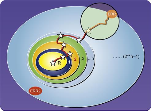
In Figure 10.5, each star represents an intermediate waypoint, a cover point fed iteratively to the tool by the user, with the red path marking the execution trace that is generated as a pseudo-reset for FPV. The black circle represents the subspace that is exhaustively searched for assertion failures by the FPV tool, showing that error condition ERR will be found, even though it is much deeper than the tool was able to explore by default. However, since the other error condition ERR2 is reachable only by a very different execution path than the user focused on, it will not be discovered by this method.
While semiformal verification sacrifices the fully exhaustive search of full proof FPV, it is still a very powerful validation method: it is equivalent to running an exponential number of random tests in a small region of the state space. Thus, if you suspect deep bugs that are triggered by a condition that you cannot exercise with your current proof bounds, you should strongly consider using this method.
In addition, be sure to examine the features offered by your verification tool; many modern FPV tools offer some degree of automation for semiformal verification. Your tool may allow you to directly specify a series of waypoints, without having to manually extract each trace and convert it to a reset sequence.
Incremental FEV
Suppose you have successfully run full proof FPV on a complex design and have been continually running regressions on it, but the regressions are very time consuming. In some cases, we have seen at Intel, we have been able to use advanced complexity techniques to successfully verify a unit, but the FPV ultimately takes several weeks to run, due to high complexity and a large number of cases that have been split.
Then a new customer request comes in and you need to modify your RTL. Do you need to rerun your full set of FPV regressions? What happens if your new change further increased the design complexity and your original FPV regressions now crash or fail to complete after several weeks?
In cases where you have changed a design that had a difficult or complex FPV run, you should consider doing an incremental RTL-RTL FEV run instead of rerunning your FPV regression. Assuming you insert your change carefully and include a “chicken bit,” a way to shut off the new features, you do not really need to re-verify your entire design. Just verify that the new design matches the old one when the new features are turned off; if you were confident in your original verification of the old model, this should be sufficient. Then you only need to write and prove assertions specifying the newly added features, which might take up significantly less time and effort than rerunning your full proof set on the entire model. We have seen cases at Intel where a formal regression that took several weeks could be replaced with a day or two of FEV runs.
Helper Assumptions … and Not-So-Helpful Assumptions
Now that we have reviewed the basic complexity techniques that should be in your toolkit, it is time to look at a few more advanced ones. One idea you should consider when running into complexity issues is the concept of helper assumptions: assumptions that rule out a large part of the problem space, hopefully reducing the complexity and enabling model convergence. This is illustrated in Figure 10.6.

In Figure 10.6, the yellow part of the cone of influence of a property has been ruled out by helper assumptions, reducing the logic that must be analyzed by the formal engines.
Writing Custom Helper Assumptions
As with many aspects of FV, the most powerful aid you can give to the tools comes from your insight into your particular design. Are you aware of parts of the functional behavior space that do not need to be analyzed in order to prove your design is correct? Do implicit design or input requirements theoretically eliminate some part of the problem space? If so, write some assumptions to help rule out these cases.
Some of the starting assumptions we have created in previous chapters, such as restricting the opcodes of our ALU or setting scan signals to 0, can be seen as simple examples of helper assumptions. Looking at our memory controller example, let’s suppose we have added our cut point at the RAW hazard computation. We know the RAW hazard can only logically be true when a read operation is in progress, but there is nothing enforcing that condition once the cut point is there—it is possible that our FPV engine is wasting a lot of time analyzing cases where a nonread operation triggers a RAW hazard. Thus, an assumption that a RAW hazard only occurs on a read operation might be a useful helper assumption.
If you are facing a complexity issue, you should think about the space of behaviors of your design, and try to find opportunities to create helper assumptions that would rule out large classes of irrelevant states.
Leveraging Proven Assertions
If you are working on a design where you have already proven a bunch of assertions, and only some small subset is failing to converge, this may provide a nice opportunity to grab a bunch of “free” helper assumptions. Most modern FPV tools have a way to convert assertions to assumptions. Use these tool features to convert all the proven assertions to assumptions—you can then leverage them as helper assumptions for the remainder of the proofs. Some tools will do something like this automatically, but even if your tool claims to have this feature, don’t take it for granted—it may be that some of your “hard” proofs started before all your “easy” proofs were completed, so many complex proofs may not be taking advantage of all your proven assertions. Thus, starting a new run with all your proven assertions converted to assumptions may provide a significant advantage.
If you are using one of the modern assertion synthesis tools, which can auto-generate some set of assertions, this may provide additional easily proven properties that you can use as helper assumptions. But avoid going overboard and creating too many assumptions or you may face the problem mentioned in the next subsection.
Do You have too Many Assumptions?
Paradoxically, although assumptions help to fight complexity by ruling out a portion of the problem space, they can also add complexity, by making it more compute-intensive for the FV engines to figure out if a particular set of behaviors is legal. You may recall that we made the same point in the context of FPV for post-silicon in Chapter 7, since it is common for post-silicon teams to have too many assumptions available due to scanout data. Figure 10.7 provides a conceptual illustration of why adding assumptions can either add or remove complexity. While a good set of assumptions will reduce the problem space, large sets of assumptions might make it computationally complex to determine whether any particular behavior is legal.

Thus, you need to carefully observe the effects as you add helper assumptions, to determine whether they are really helping. Add them in small groups and remove the “helpers” if it turns out that they make performance worse.
In addition, you may want to look at your overall set of assumptions, and think about whether they are all truly necessary: were they added in response to debugging counterexamples during wiggling, in which case they probably are essential, or were they just general properties you thought would be true of your interface? For example, one of our colleagues reported a case where he removed an assumption in the form “request |-> ##[0:N] response”, a perfectly logical assumption for an interface—and a formerly complex proof was then able to converge. Even though he was now running proofs on a more general problem space, where time for responses is unbounded, this more general space was easier for the FPV engines to handle.
Generalizing Analysis Using Free Variables
The concept of a free variable is actually nothing new: it is quite similar to a primary input, just a value coming into your design that the FV engine can freely assign any value not prohibited by assumptions. A free variable is different in that it is added as an extra input by an FPV user, rather than already existing as an actual input to the model. Usually you would create a free variable by either adding it as a new top-level input to your model, or declaring it as a variable inside your model and then using commands in your FPV tool to make it a cut point.
Free variables provide a way to generalize the formal analysis, considering cases involving each possible value of the variable at once. When the model contains some level of symmetry to be exploited, these variables can significantly increase the efficiency of formal analysis.
Exploiting Symmetry with Rigid Free Variables
Let us consider a variation of our MRA unit where it maintains tokens for various requestors and grants them according to the priority. We want to prove one property for each requestor if the tokens are granted to them based on the requirement.
parameter TOKEN_CONTROL = 64;
generate for (i=0;i<TOKEN_CONTROL; i++) begin
ctrl_ring(clk,grant_vec[i], stuff)
a1: assert property (p1(clk,grant_vec[i],stuff))
end
endgenerate
Since we placed the assertion inside the generate loop, we would end up proving slightly different versions of the assertion 64 times, which is not an optimal solution. This may result in significant costs within our FPV tool, in terms of time and memory. Is there a better way to do this? This is where a free variable can make a huge difference. We can remove assertion a1 from the generate loop and instead prove the property generally with a single assertion:
int test_bit; // free variable
test_bit_legal: assume property
(test_bit>=0 && test_bit<64);
test_bit_stable: assume property (##1 $stable(test_bit));
a1: assert property (p1(clk,grant_vec[test_bit],stuff));
As you can see above, using the free variable test_bit makes the assertion general: instead of analyzing each of the 64 cases separately, we are telling the FPV tool to complete a general analysis, proving the assertion for all 64 possible values of test_bit at once. Many FPV engines work very well on such generalized properties. If there is symmetry to exploit, with all 64 cases involving very similar logic, the FPV tools can take advantage of that fact and cleanly prove the assertion for all bits at once.
We need to be careful when using free variables, however. In the above example, we added two basic assumptions: that the free variable takes on legal values, and that it is a stable constant for the proof. You will usually need such assumptions when using free variables to replace generate loops or similar regular patterns.
Other Uses of Free Variables
The example above is one of the simpler cases of using free variables, to generalize analysis of each iteration in a large loop. Another common usage of free variables is to represent a generalized behavior, where some decision is made about which of several nondeterministic actions is taken during each cycle of execution. For example, a free variable can be used to represent indeterminate jitter at a clock domain crossing boundary, or the identity of a matching tag returned in the cache for a memory controller. Again, look for cases where multiple behaviors are handled by the same or symmetric logic, which can be exploited by FPV engines.
When using a free variable in one of these cases, you will probably not want to assume that it is permanently constant as in the rigid example above. Instead, you need to add assumptions that define when changes may occur.
In some cases, free variables can also be tough for convergence, even with similar pieces of logic applied across the bus width. It might be imperative to use case-splitting across the free variables for better convergence, while not compromising on the exhaustiveness. In the above defined logic if adding a free variable to replace 64 bits results in greater complexity, perhaps we can split the data bus into four 16-bit representations and allow the FV tool to run parallel sessions on these four care sets.
(top_freevar == 0) |-> (freevar>=0 && freevar <=15)
(top_freevar == 1) |-> (freevar>=16 && freevar <=31)
(top_freevar == 2) |-> (freevar>=32 && freevar <=47)
(top_freevar == 3) |-> (freevar>=48 && freevar <=63)
This method of splitting the cases, along with the free variable technique to exploit symmetry, can greatly simplify proving properties on complex logic.
Downsides of Free Variables
Although adding a free variable can often improve efficiency, remember that like assumptions, free variables can be a double-edged sword. When there is symmetry to exploit, this technique is a very powerful way to exploit it. But if you have an example where generalizing the analysis causes FPV tools to try to swallow multiple dissimilar pieces of logic all at once, the free variable is probably the wrong choice. You may want to choose case-splitting, running truly separate proofs for the different parts of the design space, instead.
Also, keep in mind that free variables will make your assertions and assumptions less useful in simulation or emulation. If you are planning to reuse your FV collateral in these environments, you will need to carefully add simulation-friendly directives to randomize your free variables, and even then will only get a small fraction of the dynamic coverage you would get from other properties. This is because the random values chosen for free variables will only rarely coincide with those driven by simulation.
Abstraction Models for Complexity Reduction
Abstraction is one of the most important techniques for scaling the capacity of FPV. In this context, abstraction is a process to simplify the DUT or its input data while retaining enough of the significant logic to have full confidence in our proofs. Many of the previous techniques we have discussed, such as blackboxing, cut points, and free variables, can be considered lightweight abstractions. Most abstraction models make use of free variables. However, now we are discussing more complex abstractions, where we remodel more of the logic to simpler versions that can help us overcome complexity barriers.
There are many ways of abstracting a design. Some of the most common types of abstractions are:
• Localization: Eliminate logic that is probably irrelevant to your proofs, such as by adding cut points or blackboxes.
• Counter abstraction: Instead of accurately representing a counter, create a reduced representation of its interesting states.
• Sequence abstraction: Represent an infinite traffic sequence by analyzing behavior for a small set of generalized packets.
• Memory abstraction: Represent a memory with a partial model that only accurately tracks certain elements.
• Shadow models: Choose a subset of some block’s logic to model, and allow arbitrary behavior for the unmodeled regions.
Because most abstractions significantly simplify the model, you need to keep the issue of false negatives in mind: any bug found may or may not apply to the real model, so you need to double-check potential bug finds against the actual design. You also need to be careful of false positives: as you will see below, while the majority of abstractions are generalizing the model and thus safe in the same way as cut points or blackboxes, some are naturally coupled with assumptions that limit behavior and can hide bugs.
Now we will look at examples of some of the basic types of abstractions.
Counter Abstraction
One common cause for complexity is because of the large sequential depths owing to counters. The state space diameter of the design is large in the presence of deep counters, and even worse when there are multiple counters whose outputs can interact: formal analysis may have to reach depths proportional to the product of the counter sizes to handle all possible combinations. As a result, FV of designs with counters can be complex, and is very likely to contain cover points (and thus potential assertion failures) that are not reachable by any feasible bounded proof. Moreover, the scenarios or counterexamples generated by the FV tool tend to be very long and difficult to understand.
One simple way to deal with counters in the verification process is to ignore how the counter should count and simply assign arbitrary values to the counter; this can be easily done by blackboxing the counter or making its output a cut point. In many cases, however, specific values for the counters and the relationships among multiple counters are vital to the design. Therefore, assigning arbitrary values to counters during the verification process may result in unreliable verification. So, we need to see the effect of counter values on the downstream logic before abstracting them out.
Many useful checks can be proved by replacing the counter with a simple state machine model, abstracting the state graph of an N-bit counter to a few states such as: 0, 1, at-least-one, at-least-zero. If you can identify particular values where the counter performs interesting actions, you may find that creating specific states for these makes it easier for the formal tool to quickly reach interesting model states. An example of a counter abstraction is depicted in Figure 10.8.

In Figure 10.8, when in the reset state, the model nondeterministically (based on whether a free variable is 0 or 1) decides each cycle whether to stay in that state or transition to the next state. The simplest types of counter abstractions might only represent the reset state, indicating a noncritical value of the counter, and one critical state, representing a counter value that triggers some action by a design.
Figure 10.8 depicts a counter abstraction model where several critical states are determined by the downstream logic. There are two critical states in the figure, n and m. To use this kind of abstraction, you basically need to make the original counter output a cut point, model your abstract state machine and your free variable, and then add assumptions that the original counter output always matches the output of your state machine.
The abstraction model of the counter has significantly fewer states than the counter itself, thereby simplifying the counter for the verification process. Some commercial tools now support built-in counter abstraction as a part of their offerings, making this method much easier to use than in the past.
Sequence Abstraction
In case of data transport modules, the prime responsibility of the design is to faithfully transfer the data. Sequence abstraction aims at replacing an infinite set of possible data sequences by a small set of generic representatives. The complexity for this kind of transporter arises from the properties written to check that the sequence of the incoming packets is maintained at the output.
Figure 10.9 demonstrates a mechanism to verify a design by replacing all possible packets with three distinct, but otherwise unspecified, packets, C, B, and A. We use a set of rigid free variables to define these generic arbitrary packets, constrain the inputs with assumptions stating that sequences may consist only of these packets, and then check that all possible input sequences are replicated at the output. Using this method, we can check for cases where a packet is dropped, replicated, reordered, or corrupted.

Since we are using free variables to allow arbitrary contents of our three target packets in each run, our proofs are very general, covering any kind of behavior that can be generated by continuous traffic consisting of three arbitrary (but constant) packets. Note, however, that this simplification can hide some potential bugs. For example, suppose a sequence of six distinct packet values, with no two being equal, causes some internal state machine to get into a bad state. This case will be missed, since we are only allowing a total of three distinct packet values.
This abstract model is capable of representing a large class of potential behaviors, and is likely to enable verification of a data transport model with high confidence. You do need to keep the limitations in mind, however, when deciding whether you can consider such a proof sufficient if your requirement was for full proof FPV; you should have a strong argument for why your limited number of packets should be sufficient to explore the behaviors of your design.
We should also mention that there are some other related forms of sequence abstraction (see [Kom13], for example) where rather than limiting the data that is allowed to arrive, you allow all possible data, but carefully set up your assertions to only track data that matches a small set of tags. This enables a more general analysis, sometimes with the expense of higher verification complexity.
Sequence abstractions are strong enough to represent a wide gamut of sequences and are very useful on data transport designs. Some commercial tools include the sequence abstraction mechanisms as a part of their offerings, thereby allowing the users converge faster on their data transfer designs.
Memory Abstraction
Memories, caches, or deep queues are virtually guaranteed to create complexity for FV tools, since they are basically gigantic collections of state elements. For example, a small register file with 16 entries of 64 bits each would roll out to 1,024 state elements, each of which could potentially take on new values during any clock cycle. On the other hand, memories are very regular structures, and we can usually trust that the memory itself is verified separately through specialized techniques. Thus, it is often pragmatic to blackbox memories for FV purposes, and trust that they will be verified elsewhere.
However, we cannot always safely blackbox a memory and still obtain FV proofs. Some of our properties may depend on seeing a value written to memory and then having the same value retrieved; if we completely blackbox the memory, wrong values will potentially be seen for every memory read. Thus, we need some way to functionally represent the memory in our FV environment.
A simple solution is to use parameters to reduce the memory size, as discussed in the section on parameters and size reduction earlier in this chapter. If the memory is read-only, as in a store for preprogrammed microcode, an alternative solution is to replace it with a simple module containing a large set of constant assignments rather than true state elements. Sometimes these solutions will not be sufficient, however, and a more powerful abstraction method must be used to provide a simpler representation of the memory that does not cause complexity for formal engines.
One useful way of abstracting memory is by replacing it with a new version that has a small set of “interesting” locations. For example, suppose we know that even though we have a large memory in our model, our assertions only related to operations using four memory elements at a time. Instead of worrying about all the memory entries, we define a memory that is only concerned about four entries, Entry_1 through Entry_4, as shown in Figure 10.10.
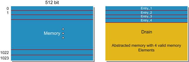
The basic interfaces for the memory would still be maintained, but we only accurately represent the memory for four particular arbitrary locations, to be represented by free variables. Our abstracted module might contain code something like this:
// free variables, will define as cut points in FV tool commands
logic [11:0] fv_active_addr[3:0]; // rigid vars for active address
logic [63:0] fv_garbage_data; // supplies random data
logic [63:0] ABSTRACT_MEM[3:0]; // The abstracted memory
logic garbage; // 1 if outputting garbage
// Keep active_addrs constant during any given run
active_addr_rigid: assume property (##1 !$changed(fv_active_addr));
always @(posedge clk) begin
for (int i=0; i<4; i++) begin
if ((op==WRITE) && (addr == fv_active_addr[i]))
ABSTRACT_MEM[i] <= din;
if ((op==READ) && (addr == fv_active_addr[i]))
dout <= ABSTRACT_MEM[i];
end
if ((op==READ) && (addr != fv_active_addr[0])
&& (addr != fv_active_addr[1])
&& (addr != fv_active_addr[2])
&& (addr != fv_active_addr[3])
) begin
dout <= fv_garbage_data;
garbage <= 1;
end else begin
garbage <= 0;
end
end
Now, instead of tracking all the entries, our accesses are limited to just four interesting entries. The abstraction is independent of the memory size and we can achieve a huge memory reduction. The complexity of the memory accesses is limited to just tracking four entries. Since these are arbitrary entries, addressed by free variables that can take on any legal value, this does not hurt the generality of any proofs that only involve four memory locations. Any accesses to other locations will return arbitrary “garbage” values.
Once we have modeled the memory, we may also need to make sure our assertions will only make use of the selected addresses, either by adding new assumptions or by adding assertion preconditions. These assumptions are not strictly required, but may be needed to avoid debugging many assertion failures due to memory reads to nonmodeled addresses that return garbage values. If we have created a signal to indicate when a nontracked memory address was accessed, like garbage in the code example above, this is fairly simple:
// Make sure address used matches a modeled address
no_garbage: assume property (garbage == 0);
In some cases, you also might want to return a standard error value for such garbage values, say 32’hDEAD_BEEF, so that you can always check for the error condition with a standard signature. When we try to create such a standard garbage value, we would have to add a constraint on the input not to feed in such a value.
Be careful when using this type of abstraction. If you do have properties which depend on more active memory elements in play than you have allowed for in your abstractions, you might find that your new assumptions or preconditions have overconstrained the environment and hidden important behaviors, creating a risk of false positives. Always be careful to combine this type of abstraction with a good set of cover points.
We should also mention here that some vendors have provided toolkits for automatic memory abstraction, so be sure to look into this possibility before implementing such an abstraction from scratch. This may save you significant effort.
Shadow Models
The final form of abstraction we want to discuss is really a catchall for a large class of design abstractions not otherwise covered in this chapter. If you have a particular submodule that is causing complexity issues, you might want to think seriously about replacing it with a shadow model, an abstract replacement model that encompasses some but not all of the functionality, using free variables to replace real and complex behaviors with arbitrary simple ones. The counter and memory abstractions we have discussed above can be considered special cases of this: the counter models an abstract state instead of keeping the count, and the memory only keeps track of a subset of its actual information.
Shadow models are not limited to these cases, however. Some other examples where FV users have seen this type of abstraction to be useful include:
• Arithmetic blocks: recognize that an operation has been requested and set output valid at the right time, but return arbitrary results.
• Packet processing: acknowledge completion of a packet and check for errors, but ignore decode logic and other handling.
• Control registers: ignore register programming logic, but preset standard register values, and enable the block to act like a normal Control Register (CR) block for read requests.
Overall, you should consider shadow models a very general technique. Any time you are facing a complexity issue, look at the major submodules of your design, and ask yourself whether you really need to represent the full extent of the logic. Chances are that you will find many opportunities to simplify and make FV more likely to succeed.
Summary
Complexity issues are an inherent challenge in FV, because the underlying problems that must be solved by FV engines are NP-complete. Thus, in this chapter we have explored a number of techniques for dealing with complexity and enabling your FV tools to succeed despite initial problems with runtime or memory consumption.
We began by reviewing our cookbook of simple techniques, most of which have been discussed to some degree in earlier chapters.
• Start by choosing the right battle, selecting a good hierarchy on which to run FV.
• Use the right options with your tool’s engines.
• Consider blackboxing or parameter reduction to directly reduce the model size.
• Look at opportunities for case-splitting, property simplification, and cut points.
• If focusing on bug hunting, also consider semiformal verification to reach deep states more easily.
• If verifying small changes to a model that has been mostly verified before, consider replacing FPV with incremental FEV.
Once you have gotten as far as you can with these simple techniques, it is time to consider some powerful but more effort-intensive methods.
• Helper assumptions can enable you to significantly reduce the problem space for FV engines. You also need to look at the converse problem, whether too many assumptions are actually adding rather than reducing complexity.
• Generalize analysis using free variables, which can often enable FV engines to solve your problems much more cleanly and quickly.
• Consider developing abstraction models, which can massively reduce complexity by looking at more general versions of your RTL or its input data.
By carefully using a combination of the above methods, we have found that many models that initially appear to be insurmountable challenges for FV can actually be verified successfully.
Practical Tips from this Chapter: Summary
10.1 It is recommended to first analyze your design for complexity before you begin an FPV effort. Look at the total number of state elements at the top level and in each major submodule, and try to aim for a size with fewer than 40K state elements.
10.2 Don’t panic if you have a bounded proof rather than a full proof. Make sure that the expected deep design behaviors are covered by proving a good set of cover points. A bounded proof may be fully acceptable as a signoff criterion.
10.3 Partition a large component into smaller, independently verifiable components to control the state explosion problem through compositional reasoning. But if you find during wiggling that this causes a need for too much assumption creation, consider verifying the larger model and using other complexity techniques.
10.4 Experiment with the engines offered by the tool, before you start resolving the convergence of hard properties. Many engines are optimized to work on a subset of design styles or property types; choose the right engine for the property under consideration.
10.5 If you are focusing on bug hunting or are in early stages of FPV, and expect many failures, take advantage of tool settings such as start, step, and waypoints to enable more efficient bug hunting runs.
10.6 Blackbox memories/caches, complex arithmetic or data transformation blocks, analog circuitry, externally verified IPs, blocks known to be separately verified, or specialized function blocks unrelated to your FV focus.
10.7 Look for opportunities to take advantage of symmetry and reduce the sizes of regular data structures or occurrences of repeated modules.
10.8 Make sure parameters are used whenever possible to specify the sizes of repeated or symmetric structures in RTL, so you can easily modify those sizes when useful for FPV.
10.9 Decompose the input care set into simple cases to assist convergence on your design.
10.10 When possible, split complex assertions into simpler atomic assertions, whose union would imply the original check intended.
10.11 Use cut points to free design logic and reduce complexity, in cases where you can identify large blocks of logic that are not in a blackboxable standalone module but are irrelevant to your verification. If you are having trouble identifying good cut points, generate a variables file and review the nodes involved in your property’s fanin cone.
10.12 If one of your proposed blackboxes needs a “hole” to allow a small piece of FV-critical logic to be visible, use cut points instead of blackboxing. You can declare each of the module’s outputs a cut point, except for the one whose logic you need.
10.13 If you suspect potential issues triggered by a design state that cannot be reached within your current proof bound (as detected by failed cover points), consider enhancing your bug hunting with semiformal verification.
10.14 If you have made changes to a stable design that had a time-consuming and complex FPV run, consider replacing FPV regressions with an FEV equivalence proof that your changes did not modify existing functionality.
10.15 If dealing with complexity issues, think about opportunities for “helper assumptions” that would rule out large parts of the problem space, and add some of these to your design.
10.16 If some of your assertions are passing, but others are facing complexity issues, convert your passing assertions to helper assumptions for the next run.
10.17 Monitor the changes in proof performance after adding helper assumptions, and remove them if they turn out not to help.
10.18 If you have a large number of assumptions and are facing complexity issues, examine your assumption set for ones that may not truly be necessary. Sometimes removing unneeded assumptions, even though it widens the problem space covered by FV, can actually improve performance.
10.19 Use rigid free variables to replace large numbers of assertion instances in generate loops with a single nonloop assertion.
10.20 Consider adding free variables when you need to represent one of several behaviors that will be chosen each cycle based on analog factors or other information unavailable during formal analysis, such as clock domain crossing jitter or tag hits in a blackboxed cache.
10.21 If you add a free variable and find that it hurts FPV performance rather than helping it, you are likely working on an example where case-splitting is a better option.
10.22 If you are facing complexity issues on a design with one or more counters, consider using a counter abstraction. Be sure to check for automated counter abstraction options in your FPV tool before doing this manually.
10.23 If you are facing complexity issues on a data transport design, consider using a sequence abstraction, representing or checking a small set of possible data items instead of fully general sequences of data.
10.24 If blackboxing or reducing a large memory does not work well for your design, consider implementing a memory abstraction. Also check to see if your FPV tool vendor has built such a capability directly into the tool, before implementing the abstraction by hand.
10.25 If you are facing complexity issues on a design with many submodules that cannot be blackboxed, examine the hierarchy for areas where complex logic can be abstracted to a shadow model, while still enabling the proofs of your important assertions.