
FPV “Apps” for specific SOC problems
Now that we have spent a few chapters on general-purpose FPV, we describe how the focus can be narrowed to form more specific “Apps” to solve particular problems encountered in typical SOC design flows. Reusable Protocol Verification enables proofs of common properties in well-documented protocols without reinventing them for each project. Unreachable Coverage Elimination supplements simulation by using FPV technology to rule out bad cover points. Formal Connectivity Verification enables verification of complex pin connection muxing with full coverage through FPV. Control Register FPV checks that every control register is following its specified access policies correctly, and that no two can interfere with each other. Finally, FPV-based post-silicon debug can enable quick reproduction of tricky logic sightings from a silicon debug environment.
Keywords
protocols; coverage; connectivity; control registers; post-silicon debug; unreachable
In addition to running much faster than simulation, formal apps provide exhaustive checks that expose corner-case bugs simulation might miss.
—Richard Goering, Cadence blogger
The past few chapters have focused on general-purpose formal property verification (FPV), where you create a set of assertions and cover points and use FPV tools to formally analyze their consistency with the register transfer level (RTL). As we have seen, this is a very powerful technique, and useful in several ways throughout your RTL design flow: for early design exercise, for bug hunting, for bulletproof verification of complex logic, or for replacing unit-level simulation for full validation signoff. However, there is a huge class of FPV applications that were missed in this discussion: FPV apps, or domain-specific uses of FPV that provide targeted solutions for specific problems.
What is an FPV app? The boundary between traditional FPV and an FPV app tends to be somewhat fuzzy. But as we define it, the distinguishing features of an app are:
• Specific domain: We are applying FPV to some specific part of the design process, or to some specific type of design, rather than just writing general-purpose assertions.
• Less knowledge required: Someone who does not have much experience with general-purpose FPV should find that learning and leveraging this FPV app is easier than gaining a full knowledge of FPV.
• Customizable: An FPV expert should be able to provide simple scripts, on top of existing FPV tools, that enable nonexperts to efficiently use the app. We should also be able to present the results in different ways from standard FPV, to make it more meaningful to experts in the domain of the particular app. Numerous vendors will likely have prepackaged scripts or tools that can save you this effort.
One other point we should mention is that many vendors have provided new apps that work by extending the capabilities of FPV engines. For example, some have enabled 3-valued logic and detection of X propagation, and some have developed property synthesis tools that automatically generate assertions based on simulation traces or static RTL analysis. We are not disputing the usefulness of these tools, but in this chapter, we want to focus on techniques that you can easily enable using standard off-the-shelf model-checking tools. Thus, apps that require new enhancements to core FPV engines are beyond the domain of this discussion. (If you’re curious about other types of apps, your favorite vendor will be happy to talk your ear off about these new tools.)
Even staying within the domain of simple apps that can be enabled with standard FPV tools, there are numerous ways you can use FPV to enhance productivity across the design flow. The ones we highlight are specific examples that have seen some degree of success in the industry; do not assume our particular selection means that other apps will not be of use to you as well. FPV should really be thought of as a general toolkit for interpreting and manipulating RTL logic, not just a specific point tool, and it is a key enabler for applications in many areas. In fact, we can be fairly certain that by the time you read this, someone will have presented a conference paper describing another FPV app that we had never thought of. The ones we highlight here include reusable protocol verification, unreachable coverage elimination, connectivity verification, control register verification, and post-silicon debug.
Reusable Protocol Verification
Reusable protocol verification is exactly what it sounds like: the use of FPV properties that describe a particular communication protocol. Since the protocol is reusable, we do not want to reinvent the wheel and recreate the set of protocol-defining properties with every design; we should create a set of SystemVerilog Assertions (SVAs) for our protocol once and then reuse in future designs as needed. You will want to strongly consider reusable protocol FPV in the following situations:
• You are trying to verify that a new RTL model complies with a well-defined protocol.
• You are doing general FPV on a model that has interfaces that should obey a well-defined protocol.
• You have defined a protocol, do not yet have RTL that implements it, and want to explore and sanity-check some typical protocol waveforms.
• You have defined a protocol that is highly parameterized to enable numerous configurations and want to provide a companion set of properties that share these parameters to support validation.
Before we start talking about this application of FPV, we need to mention one important point: for commonly used protocols, there is often FPV-compatible verification IP available for purchase from EDA vendors. Be sure to take a close look at the marketplace offerings before you start creating your own set of properties; otherwise, you may waste a lot of effort duplicating something that was easily available.
Assuming the above was not the case, or you did not have the budget to purchase formal protocol IP externally, you will need to define the properties yourself. In this section, we provide some basic guidelines for defining a standard property set for long-term reuse. Initially, if doing tentative FPV experimentation or design exploration, you might want to create quick and dirty properties rather than thinking about the long term. But if you are working with a protocol that is expected to appear in multiple designs, you will probably benefit significantly from following the advice in this section.
To clarify the discussion, we will describe a simple example protocol and show how we could create a set of reusable properties to go with it. This is a simple client-server protocol that obeys the following rules:
1. Each client has an 8-bit opcode and data signal going out to the server. The opcode field has a nonzero opcode when making a request.
2. The req_valid signal goes to 1 to indicate a request. The req_valid, req_opcode, and req_data remain constant until the rsp_valid signal, coming from the server, goes high.
3. The server responds to each request in a constant number of cycles, which may be between 2 and 5 depending on the implementation, as specified by SystemVerilog parameter SERVER_DELAY.
4. When the rsp_valid signal goes high, it remains high for 1 cycle.
5. One cycle after the rsp_valid signal is seen, the client needs to set req_valid to 0.
Figure 7.1 illustrates the signals involved in this protocol.

Basic Design of the Reusable Property Set
In most cases, we recommend defining any reusable property set as a standalone SystemVerilog module, which can be connected to the rest of the design using the bind construct. As we have seen in Chapter 3, the bind keyword in SystemVerilog allows a submodule to be instantiated in any module without having to modify that module’s code. Below is an example of the header code for our reusable property set, described as a standalone module.
module client_server_properties(
input logic clk, rst,
input logic req_valid,
input logic [7:0] req_opcode,
input logic [7:0] req_data,
input logic rsp_valid,
input logic [7:0] rsp_data);
parameter SERVER_DELAY = 2;
...
Note that all the signals involved in the protocol are inputs here. This will usually be the case, since we are trying to observe the behavior of the protocol, not actually modify any behaviors of the design.
Another important detail of this design is the use of a SystemVerilog parameter to represent aspects of the protocol that may hold multiple possible values, but are constant for any given implementation. We could have made server_delay an input instead of a parameter, but this would potentially allow it to change at runtime in some implementation, which is specifically disallowed by the rules of the protocol. Another option would be to make it an input and use an assumption to hold it constant, but since each individual protocol-using product is likely being designed based on a single specified value, a parameter seems like a more natural choice here.
Once we have fully defined the module, we need to bind it with the design under test (DUT). We could be checking an RTL model of the client, of the server, or of the full system; in the next section we discuss some complications this can cause. But assuming for illustration purposes that we want to connect these properties to the module client_model, we could do it using a bind statement like this:
bind client_model client_server_properties (.*);
Note that the use of .* assumes that we have set the names of each interface signal to be the same in both our property module and in the design module client_model. If we have changed any signal names, we would need a standard set of port mappings in the form .<port>(<signal>), as in any submodule instantiation.
The above bind will create the same effect as if we had instantiated our module inside the design module.
Property Direction Issues
Now that we have described the outline of the module, we need to start writing the properties. But as we begin to write them, we encounter a basic issue: should they be assertions or assumptions? For example, rule 1 tells us “The opcode field has a nonzero opcode when making a request.” Which of the following is the correct implementation of this rule?
rule_1a: assert property (req_valid |-> req_opcode != 0) else $display(“opcode changed too soon”);
rule_1b: assume property (req_valid |-> req_opcode != 0) else $display(“opcode changed too soon”);
A bit of reflection will reveal that either of these might be correct. There are numerous modes in which we may want to use our properties:
• Verifying an RTL model of a client. In this case, the client generates the req_opcode signal, so we should be trying to prove this property as an assertion.
• Verifying an RTL model of the server. In this case, we should provide assumptions of correct client behavior, so this property should be an assumption.
• Testing an RTL model of the full system. In this case, we want to test both sides, so the property should be an assertion.
• Exploring the protocol itself. This means we are looking for the kind of waveforms that result when assuming correctness all our properties. In this case, we need to make the property an assumption.
The best answer is that the property might need to be either an assertion or assumption, depending on the particular application of our property set. One method we can use to provide this flexibility is through SystemVerilog parameters and macros. We need to add some parameters to define the mode in which we are building the property set, then use these flags to decide whether each property is an assertion or assumption, as in the following example:
parameter CLIENT_IS_DUT = 1;
parameter SERVER_IS_DUT = 0;
parameter SYSTEM_IS_DUT = 0;
parameter THIS_IS_DUT = 0;
`define CLIENT_ASSERT(name, prop, msg)
generate if (CLIENT_IS_DUT | SYSTEM_IS_DUT) begin
name: assert property (prop) else $error(msg);
end else begin
name: assume property (prop) else $error (msg);
end
endgenerate
`define SERVER_ASSERT(name, prop, msg)
generate if (SERVER_IS_DUT | SYSTEM_IS_DUT) begin
name: assert property (prop) else $error(msg);
end else begin
name: assume property (prop) else $error (msg);
end
endgenerate
Once we have this basic infrastructure defined, our property then becomes:
`CLIENT_ASSERT(rule_1, req_valid |-> req_opcode != 0,
“opcode changed too soon”);
Now, by choosing the proper set of parameter values to pass into our property module when invoking it, we can set up our bind statement to enable testing of the client RTL, server RTL, both, or neither. The properties for the remainder of our rules are then relatively straightforward to define, as long as we are careful to recognize which side is responsible for implementing each requirement:
`CLIENT_ASSERT(rule_2a, $rose(req_valid) |=> (
($stable(req_valid)) [*SERVER_DELAY]),
“request changed too soon”);
`CLIENT_ASSERT(rule_2b, $rose(req_valid) |=> (
($stable(req_opcode))[*SERVER_DELAY]),
“request changed too soon”);
`CLIENT_ASSERT(rule_2c, $rose(req_valid) |=> (
($stable(req_data))[*SERVER_DELAY]),
“request changed too soon”);
`SERVER_ASSERT(rule_3, $rose(req_valid) |=>
##SERVER_DELAY rsp_valid,
“rsp_valid failed to rise”);
`SERVER_ASSERT(rule_4, $rose(rsp_valid) |=>
$fell(rsp_valid),
“rsp_valid held too long.”);
`CLIENT_ASSERT(rule_5, $rose(rsp_valid) |=>
$fell(req_valid),
“req_valid held too long.”);
Note that for the rule 2 properties above, we also followed one of the tips in our earlier chapters and expressed the complex property as multiple simple properties, to separately check the stability of each field. This will likely make debug much simpler in cases where the assertions fail in simulation or FPV.
Verifying Property Set Consistency
Now that we have created an initial property set, we need to ask the question: is this property set consistent? In other words, does it enable the behaviors we associate with our protocol, in expected ways? We need to have a good answer to this question before we start binding it to RTL models for verification purposes. To do this, we need to prepare a self-checking environment where we will observe cover points and prove assertions implied by our protocol.
First, as with any FPV effort, and as discussed in the previous three chapters, we need to create a good set of cover points. In this case, there are a few obvious ones to start with:
req_possible: cover property (##1 $rose(req_valid));
rsp_possible: cover property (##1 $rose(rsp_valid));
req_done: cover property (##1 $fell(req_valid));
Note that we added an extra ##1 to the beginning of each of these, to avoid false coverage success due to possible bogus transitions at the end of reset, since it is likely that these external inputs would be unconstrained during reset.
We should also create more detailed sequence covers, so that we can see that our vision of the full flow of our protocol is possible. Often these will be inspired by waveforms we have seen in the specification. One example for our case might be:
full_req_with_data: cover property (($rose(req_valid) && (req_data != 0)) ##SERVER_DELAY $rose(rsp_valid) ##1 $fell(req_valid));
We also should create some additional assertions: properties we believe to be implicit in our protocol, which should be assured if our other properties are implemented correctly. These will be only for checking our checker, so they should be protected in a section of code that will be ignored except when the checker itself is the verification target. For example, in our protocol, we know that if the opcode changes, it cannot be during a valid request, so we might create the following assertion:
generate if (THIS_IS_DUT) begin
self_check1: assert property ($changed(opcode) |->
!$past(req_valid));
end endgenerate
Now we have sufficient infrastructure that we can run our FPV tool on our property set module standalone, under the THIS_IS_DUT configuration. All our protocol-defining properties will be assumptions, so we will generate the space of behaviors that are permitted by our protocol. We can then view the cover traces and check the assertion proofs, to be sure that our set of properties is defining our protocol properly. We should spend some time looking at the generated cover waveforms, and make sure they are correctly depicting the protocol envisioned in our specification. If we see that some of the cover points are unreachable, or reachable only in ways we did not anticipate, this will indicate that there is some flaw or inconsistency in our property set that we need to further investigate.
Note that this self-consistency environment can also serve another purpose: it is a way to examine the behavior of our protocol independent of any particular RTL implementation. This can be very valuable in early protocol development and also can be a useful way to experiment with potential changes to the protocol before dealing with the complications of RTL. It can also help with judging whether behaviors described in external bug reports are truly permitted by the protocol, leading to better insight as to whether there is a core protocol bug or an issue with a particular RTL implementation. Thus, we strongly recommend that you closely collaborate with your protocol architects when developing this kind of property set and make sure to leverage it for future protocol analysis as well as RTL verification.
Checking Completeness
Another question that needs to be answered about any protocol property set is: is it complete? Does it fully capture the intent of the protocol? In many cases, this question cannot be answered except by a human who understands the protocol: most protocols we have seen are defined by plain English specifications, rather than something formal enough to be directly translatable into a set of assertions. In fact, we cheated a bit when we stated the requirements in terms of a set of well-specified rules a few subsections back. It is more likely that our requirements would initially arrive in a form something like this:
When the client sends a request, as indicated by the rise of the req_valid signal, the server waits an amount of time determined by an implementation-dependent delay (which shall be between 2 and 5) to respond with a rsp_valid signal….
At first glance, it might appear that we are stuck with having to manually translate specifications into discrete rules for the purpose of creating assertions. However, if you can convince your architects and designers to annotate the specification, it might be possible to do slightly better. The idea is to add some known marker text, along with a stated rule, to parts of the specification that would indicate a potential assertion. If you are using a word processor with an annotation feature, you can avoid messing up the text directly. For example, the first sentence above would be connected to an annotation:
RULE rsp_valid_delay: rsp_valid rises within 2 to 5 cycles (constant for each implementation) after req_valid.
Each rule annotated in the specification has a tag, rsp_valid_delay in this case. Then we just need to ensure, using a script, that each tagged rule in the specification has a corresponding tagged assertion (with assertion tags indicated in a comment line above each assertion) in the property module. One SVA assertion might cover several rules from the specification, or several might cover the same rule; this is acceptable as long as each rule is covered. For example:
// RULES: rsp_valid_delay, opcode_valid_data_const
`CLIENT_ASSERT(rule_2a, $rose(req_valid) |=> (
($stable(req_valid)) [*SERVER_DELAY]),
“request changed too soon”);
`CLIENT_ASSERT(rule_2b, $rose(req_valid) |=> (
($stable(req_opcode))[*SERVER_DELAY]),
“request changed too soon”);
`CLIENT_ASSERT(rule_2c, $rose(req_valid) |=> (
($stable(req_data))[*SERVER_DELAY]),
“request changed too soon”);
This method will not ensure total completeness—there is still a major human factor involved—but it does help ensure that your property module will attempt to cover each of the rules thought important by the protocol architects.
Unreachable Coverage Elimination
The next FV app we discuss is unreachable coverage elimination (UCE). UCE is the method where we examine coverage goals that simulation has failed to reach despite many runs of random testing and try to use FPV to identify theoretically unreachable ones so they can be eliminated from consideration. In other words, we are using FPV to aid our analysis of simulation efforts, rather than as an independent validation tool in itself. You should consider running UCE in cases where:
• Your primary method of validation is simulation, and you have coverage goals that simulation is failing to reach.
• You want to automatically eliminate as many cover points as possible before starting manual review and test writing to cover the missing cases.
In the simplest case, where your coverage is defined by SVA cover points in the RTL code, running UCE is really just the same as doing targeted FPV runs. Just choose the parts of your design containing unreached cover points, and launch a standard FPV tool on those. You do need to be careful about choosing hierarchy levels at which your FPV tool can load the model.
Running FPV for UCE purposes is much easier than doing “real” FPV runs as discussed in Chapters 5 and 6, because you do not need to worry as much about writing assumptions. The reason is that assumptions narrow the space of possible behaviors of your design, so running without them in UCE is a conservative choice. If you run without assumptions, you are being overly generous in the behaviors allowed—which means that if some cover point is unreachable even in this case, you are certain that it is globally unreachable. Figure 7.2 illustrates this situation.
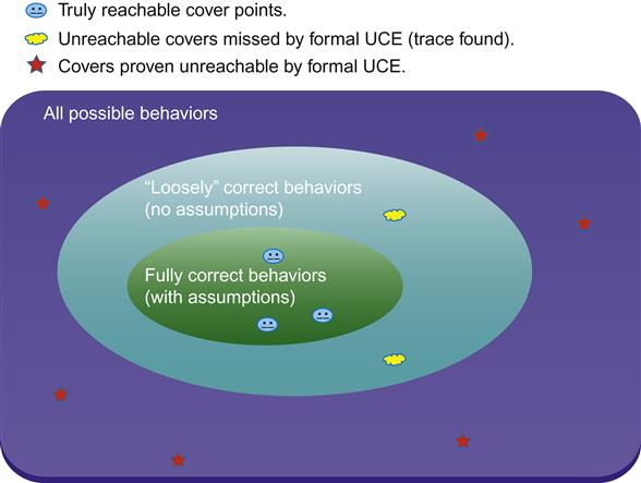
We can see that although some unreachable cover points may not be caught without a full set of FPV assumptions, there is still a good chance that many will be caught without them. The key point is that we minimize the danger of throwing out a good cover point, since we are exploring a space wider than the real behaviors of our design. However, we do need to take care to use a reasonable definition of the design’s clocks and reset for our formal runs; you will likely find that a reset trace from simulation is a good FPV starting point. Overall, a good strategy on a project that is having trouble achieving simulation coverage is to do lightweight FPV runs on major blocks, and use these to identify an initial set of unreachable cover points.
Once a cover point is found unreachable, you need to further examine it to decide if that matches the design intent. In many cases, an unreachable cover point may be part of an old feature or block that was inherited in the RTL, but is not part of the currently intended functionality, and can be safely eliminated from the list of coverage targets. If, however, the designers believe that the point should be reachable, then the unreachable cover may indicate a real design bug. In that case, you probably want to debug it with FPV to better understand why your cover point cannot be reached, as we discussed when talking about cover points in Chapter 6.
The Role of Assertions in UCE
While we can get some decent information from a simple assumption-free UCE FPV run, we can do even better if we are using a design that contains assertions. Since our premise is that if you are doing UCE, you are late in the project cycle and trying to close simulation coverage, we are probably safe in assuming that you have high confidence (resulting from many simulation runs) in the assertions that are present in your code. Since this is the case, we can create a much better UCE FPV run by converting many of those assertions to assumptions. Most modern FPV tools have commands allowing such a conversion.
This might seem a bit strange at first, since we are likely constraining many noninput nodes for testing. But remember that in FPV, an assumption is a constraint on the universe of legal simulations: in effect, we are telling the FPV tool that in any simulation, it should only consider inputs that will result in our assertions being true. This is exactly what we want since we know that none of the valid simulation tests are violating any assertions. In effect, we have further restricted our space of possible simulations, which may now allow us to prove even more cover points unreachable, as shown in Figure 7.3.
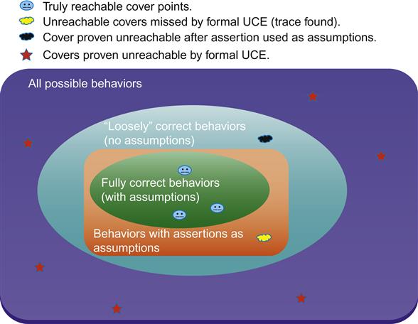
We should point out that since simulation-focused assertions are not usually created with formal rigor in mind, they are not likely to provide the full set of assumptions that defines all legal behaviors. This is why the central oval in Figure 7.3 does not coincide with the assertions-as-assumptions region around it. However, simulation-focused assertions can do an excellent job of constraining the behaviors considered by UCE FPV and better enabling a validation team to stop wasting time trying to hit truly unreachable coverage points.
One other issue to be aware of is the fact that too many assumptions can create a complexity issue for FPV. If you find that blindly converting all assumptions to assertions creates performance problems, you may want to instead manually select an interesting subset to use in your UCE FPV run.
Covergroups and Other Coverage Types
We have focused our discussion on SVA cover points, the straightforward assertion-like coverage constructs that are automatically evaluated by any FPV tool. But what about other coverage types such as SystemVerilog covergroups, or line/statement/branch coverage? In the best case, your FPV tool will have features to evaluate these kinds of coverage as well, and detect some subset of unreachable coverage constructs, such as dead code, automatically. But in cases where it does not, you will need to consider using scripts (or manual work) to create SVA cover points logically equivalent to your other constructs.
Connectivity Verification
Formal connectivity verification refers to the usage of an FPV tool to verify correctness of the top-level connections created during assembly of multiple components, such as in the case of an SOC. The idea of using a FV tool to check connectivity might initially sound strange; in fact, the authors initially dismissed the idea when it was first broached at Intel a few years ago. Don’t most designs have simple correct-by-construction scripts that guarantee correct connectivity using methods much simpler than FPV engines?
Actually, a modern design can involve connecting dozens of independently designed IP blocks, through top-level multiplexing blocks that can direct external pins to different functional blocks, with varying delays, depending on the value of various control registers. This means that there are many corner cases where combinations of control values and pin routings interact with each other. Designers want to have strong confidence that their validation provides full coverage. Traditionally this has been addressed by simulation, but it means that many hours of simulation are required after each connectivity change to cover all cases.
FPV is an ideal solution here, since it inherently covers all corner cases, and this MUXing logic is very simple in comparison to other FPV problems. Most connectivity conditions can be converted to straightforward assertions of the form:
pin1: assert property (
(ctrl_block.reg[PIN_SEL] == 1) |-> ##DELAY
(ip_block.pin1 == $past(top.pin1,DELAY)));
Once these assertions are generated, they can often be proven in seconds on typical SOCs. This results in a major productivity difference, allowing almost instant feedback for designers instead of the previous multi-hour delay due to running a comprehensive simulation suite. Thus, connectivity FPV is increasingly being seen as an easy-to-use technique that is fundamental to the SOC assembly flow. It can be implemented using simple scripts on top of a standard FPV tool, in addition to the fact that several tools on the market offer features to support this method directly.
There are a few issues, however, that you do need to be aware of when setting up a connectivity FPV run: setting up the correct model build, specifying the connections, and possible logic complications.
Model Build for Connectivity
The first issue that you need to think about when setting up connectivity FPV is: building the model. Until now, we have emphasized in most discussions of FPV that you will typically run on a unit or partial cluster model, due to known limitations of tool capacity. However, connectivity FPV usually makes the most sense if run at a full-chip level. Fortunately, this is not usually a major obstacle, since in most cases the full-chip connectivity models can blackbox almost all logic blocks: remember that we are just verifying the paths from top-level pins to major block boundaries. Figure 7.4 illustrates a typical full-chip model after blackboxing for connectivity verification:

As you can see in Figure 7.4, most major logic blocks can be blackboxed, with only a small subset actually needed for connectivity verification.
One common mistake when first building such a model is to start by trying to build a full-chip model with no blackboxes, then blackbox what is needed for simplification. This may be a reasonable strategy with typical simulation or floor planning tools, but tends to cause major problems with FV tools. Due to the inherent limitations of FPV capacity, such a tool will often not even be able to compile an un-blackboxed full-chip model. It is much better to start by building a “shell” model, with just the top level of your chip represented and all its submodules blackboxed. Once this is built, gradually un-blackbox elements of your design that you know are participating in top-level connectivity: control registers, MUXing blocks, and so on.
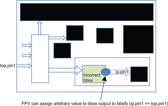
It is okay if you accidentally leave something blackboxed unnecessarily at the end of this process, since you will ultimately catch this while debugging your failing connectivity assertions. If some blackboxed element happens to fall inside a connectivity path, your FPV tool will report a bogus connectivity bug (due to treating the output of the blackboxed block as a free output), and you will discover the issue. There is no way such an extra blackbox could create a false positive, where a real error is missed. Figure 7.5 illustrates this situation.
Specifying the Connectivity
Aside from building the proper model, the other major component of the connectivity FPV setup is specifying the actual connectivity requirements. Essentially, for each top-level signal that is to be connected to the boundaries of one or more IP blocks, and each value of the relevant control registers, we need:
Most teams find it convenient to express this in some kind of spreadsheet format, as in Table 7.1.
Table 7.1
| Signal | Control register | Control value | Destination signal | Delay range | Other cond. |
| top.s1 | regblk.r1 | 0 | top.blk1.s1 | 2 | – |
| top.s1 | regblk.r1 | 1 | top.blk2.s1 | 3 | !top.scan |
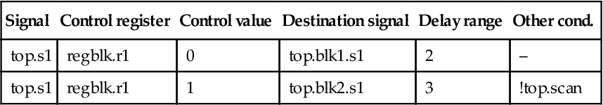
Many EDA tools define spreadsheet formats like this that can be natively read by their tools and implicitly converted to assertions, and later back-annotated during debug to simplify the overall process. However, even without such a feature, it is relatively easy to create a script that would translate the table above into assertions like the following:
s1_conn_0: assert property ((regblk.r1 == 0) |->
##2 top.blk1.s1 == $past(top.s1,2));
s1_conn_1: assert property (
(regblk.r1 == 1) && (!top.scan) |->
##3 (top.blk2.s1 == $past(top.s1,3));
These assertions can then be proven like any standard FPV assertions. The logic to connect SOC signals tends to be a rather simple set of MUXes and delay elements, so assertions like these are typically proven very quickly by most modern FPV tools.
Possible Connectivity FPV Complications
As mentioned above, the connectivity properties tend to involve very simple logic compared to typical FPV runs. However, there are still various complications that users of this type of flow have tended to encounter. The most common ones we have seen are low-level pad cells, complex interface protocols, and top-level constraints.
The first issue involves the fact that the top-level interface signals of a typical SOC design need to pass through pad cells to reach the outside world. These cells are often excluded by design teams from most RTL logic flows, because they represent very simple logic but possibly complex electrical and physical issues. Thus their authors, who are usually backend experts, tend to use nonsynthesizable SystemVerilog constructs such as explicit transistors and weak assignments. (If you usually work at a logic level like the authors, there is a good chance you have never seen these constructs. That is okay—at least one of the authors first learned about some of these while debugging connectivity FPV!) Since FPV tools cannot handle such constructs, they will result either in compilation errors or in bogus reports of combinational loops. Thus, to enable sensible connectivity FPV, you may need to replace low-level pad cell SystemVerilog modules with simpler logical representations. For example, you may see a cell like this, probably with less helpful comments:
module ugly_pad(vcc,vss,in1,out1)
// Transistor structure that doesn’t change logic
bufif1(tmp,in1,vcc);
// Weakpull for cases when pad not in use
assign (weak0,weak1) out1 = vss;
// Real action of pad
assign out1 = tmp;
end
To enable connectivity FPV, you will need to modify it so you can get a synthesizable logical view when needed:
module ugly_pad(vcc,vss,in1,out1)
`ifdef FPV
assign out1 = in1;
`else
// Transistor structure that doesn’t change
bufif1(tmp,in1,vcc);
// Weakpull for cases when pad not in use
assign (weak0,weak1) out1 = vss;
// Real action of pad
assign out1 = tmp;
`endif
end
In general, you need to be careful when modifying any logic as part of an FPV effort, but usually the logic of these types of cells is conceptually simple. Be sure to review any changes with the cell’s original author or an equivalent expert, of course, to be sure your modifications are logically sound.
The second common challenge of connectivity FPV is the issue of programming the control registers. Normally we expect that connectivity logic will be relatively simple and not require very deep reasoning by formal engines. However, if testing conditional connectivity based on control register values, there may be more complexity due to some logical protocol being needed to program the values of these registers. You may find that you already have a good set of assumptions for this protocol, especially if using a common protocol assertion set as discussed earlier in this chapter, reducing the effort needed to create more assumptions. This could still leave you with a high-effort run by the formal engines to analyze the programming of the control registers in every connectivity proof though.
A key insight that can help to address this issue is that, when doing connectivity FPV, your goal is not really to prove the correctness of the control register programming. Presumably other parts of your validation effort, either formal or simulation runs, are already focusing on this area in greater generality anyway. When running connectivity FPV, you are just trying to prove correctness of the connectivity logic. Thus, it is likely acceptable to abstract the control registers: make them cut points, telling the FPV tool to ignore their fanins and let them take on an arbitrary value, then add assumptions to hold them constant for each formal run. This way you will prove that for any given constant value of the control registers, the connectivity is correct, even though you are not spending effort in this run to prove the correctness of the register programming logic.
The last common complication with connectivity FPV that we discuss is the problem of top-level constraints. As with any FPV run, you will often find that the first time you attempt it, you will get false failures reported due to lack of assumptions. There is really nothing special about this problem in the connectivity context; the only difference is that you may need to deal with top-level mode pins that did not affect your block-level runs. Often you will have to assume that a top-level scan or debug mode is off, or that high-level “vss” and “vcc” pins actually do represent a logical 0 and 1. You may also face issues due to multiple clocks in the design; if some IP blocks use different clock domains or clocks that have passed through a blackbox, you need to correctly inform the FPV tool of their frequency in relation to the model’s main clock. Treat this like any other FPV run and work with experts in the proper area to examine your initial counterexamples and identify relevant top-level assumptions or clocking specifications.
Control Register Verification
Nearly every modern design has some set of control and status registers, addressable blocks of data that can be read or written at runtime to set major control parameters or get status about the operation of the SOC. These registers each contain several fields, which can have a variety of access policies: some are read-only, some are write-only, some can be freely read or written, and some can only be accessed if certain control bits are set. It is usually very important that these access policies are correctly enforced, both to ensure correct functionality and to avoid issues of data corruption or leakage of secure information. We also need to ensure that registers cannot overwrite or interfere with each other’s values.
Control registers can sometimes be subject to tricky errors that are hard to find in simulation. For example, suppose two unrelated read-write registers are accidentally assigned the same address, and write attempts to the two can overwrite each other. If they are unrelated, it is possible that none of the random simulation tests will happen to use both the registers at the same time, and thus it is very easy to miss this issue. As a result, it has become increasingly popular in the industry to replace simulation-based testing with FPV-based applications to exhaustively verify control register functionality. Like the connectivity problem, the control register problem is one that tends not to be as complex as other types of control logic, often enabling FPV tools to handle it very efficiently. However, there are a lot of possible combinations of operations that make exhaustive simulation-based testing inconvenient or infeasible.
A typical control register block interface is shown in Figure 7.6. As you can see in the figure, a control register block is usually accessed by providing some kind of opcode indicating a read or write operation, an address and data for the transaction, and some kind of security code (usually generated elsewhere on the chip) to signal the type of access that is authorized. There is also a bit mask to limit the access to specific subfields of a register. Typical outputs include a data out bus, to service requests that read data, and an error flag to signal that an illegal access was attempted.

Most modern FPV tools provide optional apps to directly handle control register verification, often with support for the emerging IP-XACT specification language (see [IEE09]), but in any case it is relatively easy to write scripts to set up the FPV run directly. You just need to design an input format that represents the expectations of your control registers and convert this into SVA assertions.
Specifying Control Register Requirements
Typically, a simple spreadsheet format can be used to specify the requirements on control registers. For each register, you need to specify
Then, for each field, you need
There are a number of access types supported for typical registers. Here are some of the most common ones:
• Read-Write (RW): Register can be freely read or written.
• Read-Only (RO): Register can only be read. This is often used to communicate status or hardware configuration to the outside world. (Often there is specific internal logic that can write to it, as in the fault_status example above, but through the register access interface it can only be read.)
• Write-Only (WO): Register can only be written. This is a common case when setting runtime parameters.
• Read-Write-Clear. (RWC): Register can be read, but any write attempt will clear it. This is sometimes useful if communicating status information to the outside world, and we want to provide a capability to externally reset the status.
In Figure 7.7, we illustrate a few lines of a typical control register specification spreadsheet.

In this example, we have two registers, each with two fields. The first, ARCH_VERSION, is at address 0010 and has security authorization code 05. It has two 16-bit fields. The arch_major field, with default value 1, is RO, probably used to communicate a hardcoded chip version to the user. The os_version field is RW, probably so it can be modified by software, and has default value 7. The second, FAULT_LOGGING, is a 17-bit register at address 0020 with security authorization code 01. It contains a 16-bit fault_status, through which the design can communicate some status information to a user, with default value 0. Its type is RWC, so the user can clear it with a write attempt. It also contains a WO fault_logging_on bit, through which a user can activate or deactivate fault logging, defaulting to 1.
We should probably comment here on why there is a spot in the table in Figure 7.7 for the internal RTL signal for each register. If we are trying to verify correct accesses through the register interface as shown in Figure 7.6, why should we care about the internal nodes? While verifying externally is the ideal, we need to keep in mind the fact that for many register types, there are major limitations to what we can verify through the external interface. For example, if a register is WO, we can never externally see the result of the write that sets its value, so what kind of assertion could we write on its correctness? Thus, whitebox style assertions, which look at the internal register node as part of the verification, often make the most sense for control registers.
Once you have decided on the specification of your control registers, you can use this information to generate SVA assertions.
SVA Assertions for Control Registers
There are many types of assertions that can be generated to check the correctness of control register accesses. Here we describe the ones that we typically use to check registers with the common access types described above (RW, RO, WO, and RWC). Each of the assertion classes below is generated for every applicable register and field. With each, we illustrate one of the assertions that correspond to the specification in Figure 7.7.
In general, you should be examining your company’s specification for its control registers, and generating assertions related to each defined operation for each register type. Don’t forget to include assertions both that correct operations succeed, and that incorrect operations do not modify the register value.
We are also assuming here that our design only allows writes at a field granularity (we should enforce this with separate assertions/assumptions), so we don’t have to account for messiness due to differing bit masks. Thus, for a given access attempt, each field is either totally enabled or totally disabled.
• Correct Reset Value. (All types.) We should check that each register field has the correct default value after reset.
assert property ($fell(rst) |-> cregs.rf.arch_reg[31:16] == 7);
• Always Read the Reset Value (RO). Since the field is RO, all reads should get the reset value.
assert property ((Opcode == READ) && (Addr == 0010)
&&SecurityDecode(SecurityCode,Opcode,05)
&& (BitMask[15:0] == 16’hffff) |=>
(DataOut == 1));
• Correctly Ignore Writes. (RO). After a write attempt, field value is unchanged.
assert property ((Opcode == WRITE) && (Addr == 0010)
&& (BitMask[15:0] != 0) |=>
$stable(cregs.rf.arch_reg[15:0]);
• Unauthorized Operation. (All). Security code does not allow the current operation, so flag error and don’t change register.
assert property ((Addr == 0010) &&
!SecurityDecode(SecurityCode,Opcode,05)|=>
$stable(cregs.rf.arch_reg[31:0] &&
ErrorFlag);
• Correct Value Read. (RO, RW). Reads from the designated address successfully get the field’s value.
assert property ((Opcode == READ) && (Addr == 0010)
&& SecurityDecode(SecurityCode,Opcode,05)|=>
DataOut[15:0]==cregs.rf.arch_reg[15:0]);
• Correct Value Written. (WO, RW). Writes to the designated address successfully set the field’s value.
assert property ((Opcode == WRITE) && (Addr == 0010)
&& SecurityDecode(SecurityCode,Opcode,05)
&& (BitMask[31:16] == 16’hffff) |=>
(cregs.rf.arch_reg[31:16] ==
$past(DataIn[31:16]));
• No Read from WO. (WO) A read attempt on a write-only field should result in all zeroes on the data bus.
assert property ((Opcode == READ) && (Addr == 0020) &&
(BitMask[16] == 1’b1) |=>
DataOut[16]==0);
• RWC Clears Correctly. (RWC) A write attempt correctly clears an RWC register.
assert property ((Opcode == WRITE) && (Addr == 0020)
&& SecurityDecode(SecurityCode,Opcode,01)
&& (BitMask[15:0] == 16’hffff) |=>
(cregs.rf,fault_log[15:0] == 0));
• No Data Corruption. (All) A nonwrite operation, or a write to another field or address, does not modify a field’s value.
assert property ((Opcode != WRITE) || (Addr != 0020)
|| (BitMask[15:0] == 0)) |=>
$stable(cregs.rf.fault_log[15:0]));
• Read-Write Match. (RW) If we write to the field, and we read it later on, we receive the value we wrote. This is technically redundant given the above assertions, but this lets us focus on observing the full expected flow for a RW register. It also has the advantage of being the only assertion in this set that can check write correctness without relying on whitebox knowledge of the internal register node, which may be needed in some cases where the internal implementation is not fully transparent or documented.
assign write_os_version = (opcode == WRITE) &&
(Addr == 0010) &&
(BitMask[31:16] != 0);
assign write_os_version_val = (DataIn[31:16]);
always @(posedge clk) begin
if (write_os_version) begin
write_os_version_val_last = write_os_version_val;
end end
assign read_os_version = (opcode == WRITE) &&
(Addr == 0010) &&
(BitMask[31:16] != 0);
assert property (write_os_version ##1
(!write_os_version throughout read_os_version[->1]) |=>
DataOut[31:16] == write_os_version_val_last);
The list above is not fully exhaustive, because many designs offer other register access types, locking mechanisms to limit access to certain registers, security policies that require additional inputs, and similar features. But the set of assertions we recommend here is a good starting point. Also, since most of these are expressed as triggered assertions, in most FPV tools they will automatically generate a good set of cover points showing that we can cover each typical access type.
Major Challenges of Control Register Verification
There are a number of challenges you are likely to face when setting up control register FPV. You need to properly select the verification level and the initial FPV environment for the control register FPV run. In addition, you need to account for multiple register widths and internal hardware writes.
• The Verification Level. In many cases, you might initially find it natural to run control register FPV at the level of your unit/cluster interface or at the same level as your other FPV verification environments. However, it is often the case that some complex external protocol must be decoded in order to form the simple register access requests implied by Figure 7.6. You need to consider whether you really need to be re-verifying your top-level decode logic: in most cases, this is well verified elsewhere, and there is no point in analyzing the same logic while doing control register FPV. Thus, in most cases, control register FPV is best run at the interface of a control register handling block, with interface signals like those in Figure 7.6. Naturally, you should separately ensure that the top-level decode logic is verified somewhere, either through its own FPV run or through other validation methods.
• The FPV Environment. Along the same lines as the above comment, focus on an FPV environment that just contains your register handling block. Also, be sure to remove any assumptions you created to constrain control registers in other FPV environments: these can overconstrain your control register verification, reducing the coverage of real cases, and cause your cover points to fail.
• Multiple Access Widths and Register Aliasing. In some designs we have seen, registers may be up to 64 bits wide, but the register file can be addressed in 32-bit chunks. This means that for a wide register, an access to bits [63:32] at an address A is equivalent to an access to bits [31:0] at address A+1. This requires care when writing the assertions: for example, it is no longer true that a write to a different address will not modify the register (as in our “No Data Corruption” assertion above), because a write to the next higher address can change its upper bits. There may also be cases of more general register aliasing in your design, where two registers with different logical addresses may refer to the same internal node, and you should be careful to account for such cases as well.
• Hardware Write Paths. You may have noticed that we mentioned the concept of status registers, which can be written to internally by the hardware to indicate status or events occurring on the chip. This mode of access will likely cause failures of many of the assertions above, which implicitly assume that all registers are accessed through the explicit interface in Figure 7.6. In fact, Figure 7.6 omits the detail that the hardware can internally write to registers through a separate interface; Figure 7.8 provides a revised picture that includes these.

The simplest method is to add an assumption that the internal hardware interface is inactive during control register FPV, in order to verify that the register specifications are correct with respect to the external interface. Alternatively, you can do more comprehensive verification by creating reference models of your registers that account for this alternate access path.
Post-Silicon Debug
The final application we will look at in this chapter is FPV for post-silicon debug. At first, this usage model might sound surprising, since RTL FPV is generally thought of as a pre-silicon design and validation tool. In fact, however, FPV is ideally suited for “last-mile” debug in cases where we need to diagnose and fix a post-silicon bug sighting.
As you would expect, FPV is not really useful when diagnosing lab sightings at the full-chip level, or when looking at electrical or timing issues, which are beyond the domain of RTL verification. But when you have isolated a bug to the cluster or unit level and suspect that you are dealing with a core RTL logic issue, FPV is ideally suited for reproducing and understanding the suspected bug. This is because of the principle you have seen us mention numerous times in this book: FPV lets you specify the destination rather than the journey. If a logic bug is observed in post-silicon, it is a key indicator that your validation environment was previously incomplete, so you need some tool that can find a new trace based on the observed bug.
In practical terms, this means that if you can characterize a suspected bug sighting at the RTL, in terms of a particular pattern of signal values on outputs or scanned state signals, you should be able to describe it as an SVA sequence. You can then use FPV to solve for a legal input pattern that would generate this sequence. If you succeed, then you will be able to see the bug occurring at the RTL, and you can test suspected fixes to see if they will eliminate the problem. If FPV proves that the bug pattern is not reachable, then you are able to rule out the suspected logic bug, and focus on other issues such as timing problems.
To make this discussion more concrete, let’s assume you are looking at a CPU model containing the arithmetic logic unit (ALU) from Chapter 6, reviewed again in Figure 7.9.

Furthermore, we will assume that a post-silicon sighting has been reported, where after several addition operations, the resultv output goes to 1 and outputs a bogus result during an “off cycle” when no operation is happening. Just for fun, we will also assume that this ALU is complex enough that we could not run FPV on a model containing the whole thing. How would we go about debugging this sighting with FPV?
Building the FPV Environment
We are assuming here that you have reached a point in your initial post-silicon debug efforts where you have developed a basic understanding of your defect observation, and suspect a logic bug in a particular area of your design. As with any FPV effort, you must now choose a hierarchy level in your RTL at which to run FPV. The usual capacity limitations need to be considered here, such as being unable to run at a full cluster or chip level. Of course, you should employ the standard methods used to make designs more tractable for FPV: blackboxing large memories, reducing parameters, turning off scan modes, and so forth. However, you do have a slight advantage over general FPV runs in this case: you can take into account specific characteristics of the bug you are observing. For example, you might normally be unable to run FPV at a cluster level due to the large amount of logic. But if you know from the bug you are observing that a particular functional block is involved, you may be able to blackbox unrelated blocks.
In the case of our ALU, we are told that our sighting occurs after a series of add operations. Thus, it is likely that we do not need the logical subunit, so we should blackbox this for FPV purposes. So our first step is to blackbox the logical subunit and use FPV to try to cover the point. Here we create a cover point to look for cases where the result signal is seen without having resulted from a valid ALU uop:
c1: cover property (resultv&& !$past(uopv,ALU_DELAY));
When we run this cover point, FPV will quickly come back with a waveform that shows the blackboxed logical subunit generating a logresultv value of 1. This is because, as we have seen in previous chapters, when a unit is blackboxed, its outputs are freely generated by the FPV environment. This shows that we need to add an assumption to keep the blackboxed unit quiescent and avoid bogus traces. This is a common situation when we are blackboxing large parts of the logic while chasing a specific bug: rather than a pure blackbox, we need to make sure the ignored parts of the logic are not generating bogus traces that look like our bug but are unrealistic. Just as in regular FPV runs, you should expect a few iterations of wiggling as you fix your assumptions to avoid incorrect traces.
Now suppose we have made this fix and are attempting to run our cover point c1 again, but hit an FPV complexity issue. We should take a closer look at other ways we can narrow the proof space that the FPV tool is examining. In particular, in this case we were told that a series of add operations is triggering the bug. This means that in addition to eliminating the logical subunit, we should also constrain the arithmetic subunit to only consider OPADD operations:
fv_overconstrain_add:
assume property (Uopcode == OPADD);
While this might be too overconstraining for a general-purpose proof, again we need to keep in mind that we are trying to focus on a particular bug we have observed in the post-silicon lab. In general, we should not be afraid to add very specific assumptions to help narrow down the proof space to correspond to the bug we are chasing.
Once we have added this assumption, we are focusing more directly on our suspected bug. Now when we attempt the FPV proof on our cover point, we are much more likely to be able to see a real waveform that corresponds to our problem from the lab. Once we have reproduced this in an FPV environment, it will probably be very easy to find its root cause in the RTL logic.
The Paradox of Too Much Information
One tricky issue that is sometimes faced by those performing post-silicon FPV is the paradox of having much more information than is needed. For example, suppose our debug lab has sent us a set of scan traces from our ALU, showing the values of thousands of signals over the course of thousands of cycles. In theory, we could convert these to thousands of assumptions, in line with the principle above of overconstraining our design to focus on the bug. But will this help our FPV run?
Actually, adding large numbers of assumptions can often increase the complexity of the state space, reducing rather than increasing the efficiency of FPV. While a small number of assumptions can help to reduce the problem space, having lots of assumptions can make it a more computationally difficult problem to explore that smaller space. Since we are working with heuristics and provably complex problems, there are no hard-and-fast rules here, but in general, you should avoid converting a full scan dump into FPV assumptions.
Figure 7.10 illustrates this issue in an abstract way. The oval on the left represents the full behavioral space of a design. The one in the middle shows the space with a small, clean set of assumptions: for any given point, it is fairly easy to determine whether it is in the acceptable proof space. The one on the right illustrates the situation with a complex set of assumptions. While the overall legal proof space that must be analyzed may be smaller, it now is very complex to determine whether any given behavior is inside or outside the acceptable space, due to the irregular boundaries created by the large number of assumptions.
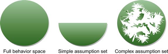
Thus, instead of blindly translating all your scan data to assumptions, use your scan dump as a source of information and just choose a handful of significant signals based on your knowledge of the most important parts of the design for your particular bug. For those signals that you have identified as important, use the scan dump values to create assumptions. It can be difficult when you do not know exactly where the bug is, but try to be sparing in your choice of significant signals, to avoid a complexity blowup due to assumption handling.
Using Semiformal Design Exploration
One other important technique you are likely to make use of in post-silicon analysis is semiformal verification. This refers to the idea of running FV starting from a known active state, a “waypoint,” rather than starting from a reset point. This makes the verification less general, but when trying to reproduce or hunt for bugs, can enable you to reach a bug much faster if the proper waypoints are chosen.
In the case of our ALU example, suppose we find that FPV always hits complexity issues after reaching a proof bound that encompasses two complete ADD operations. We can set our first waypoint to be a cover point indicating the completion of the first operation:
waypoint1: cover property ( resultv &&
$past(uop,ALU_DELAY)==OP_ADD);
When we get a cover trace for this property, we can then save that and use it as the reset phase for our next FPV run. This means we will be doing a less general analysis that full FPV—starting from the trace of one particular completed ADD operation rather than a fully general one—but this may allow the formal engine to reach a depth where it has analyzed three ADD operations instead of just two.
In cases of greater complexity, it is often beneficial to define several waypoints: use FPV to cover the first one, then use the first waypoint to start an FPV run that reaches the second, and so on. For example, perhaps we might need to define a second waypoint, indicating the completion of the next ADD operation, in order to generate a run that reaches the bug on the ALU. On some models, the use of multiple waypoints can enable successful FPV bug hunting at a significantly greater depth than might initially seem feasible.
We will discuss semiformal verification in more detail in Chapter 10, where we describe many techniques for dealing with complexity. But we highlight it here because it is a method that has shown itself to be particularly valuable in the context of using FPV to analyze post-silicon bugs.
Proving your Bug Fixes Correct
Once you have successfully reproduced a post-silicon bug by generating a trace with FPV, you will hopefully be able to examine the RTL operations involved and come up with a bug fix. Then you will face another issue, similar to the diagnosis problem but with some important differences: proving the bug fix correct. This is actually one of the really powerful arguments for using FPV in post-silicon: the ability to not only replicate a bug, but to then prove that a proposed fix really fixes the bug, for traces more general than the particular one that triggered the initial issue. As you have probably seen if you have been involved in real-life post-silicon debug challenges, it is often the case that an initially proposed bug fix for a tough post-silicon issue will overlook some detail and not be a fully general fix.
The most obvious way to check the completeness of a bug fix is to load your modified RTL into the same FPV environment that you used to diagnose the bug and make sure it proves that your bug-related cover point can no longer be reached. This is an important sanity-check, and if the models you are using are very complex for FPV, or required techniques such as semiformal verification to enable a usable run, it may be the best you can do to gain confidence in the fix. But you should not stop at this point if you can avoid it.
Remember that for diagnosing the issue, we stressed the need to overconstrain the design to focus on the particular bug. But when trying to prove the bug fix fully general and correct, you need to reexamine the overconstraints, and make sure they were each truly necessary. For example, in our ALU model, we might ask ourselves:
• Can this only happen with addition ops?
• Does the logical subunit have a similar issue to the arithmetic one?
To answer these questions, we need to either remove some of the assumptions and blackboxes or create special-case FPV environments with a different set of assumptions to check the parts of the logic we skipped: check operations other than OPADD, or switch the blackbox to the arithmetic subunit while un-blackboxing the logical one.
Conceptually, it is often much easier to generalize an FPV environment than it would be to generalize a simulation environment, when trying to provide more complete checking of a proposed bug fix. The challenge is to recognize that you need to pay extra attention to this problem; after a grueling high-pressure post-silicon debug session, there is often an inclination to declare victory as soon as FPV first passes. FPV has a lot of power, but you must remember to use it correctly.
Summary
As you have probably noticed, this chapter was a little different from the past few, in that it provided a grab bag of several different “apps” applicable at various phases of the SOC design and verification flow. We looked at methods that are applicable across the spectrum of SOC design, including:
• Reusable Protocol Verification: Creating a set of FPV-friendly properties for a common protocol that allows you to reuse verification collateral with confidence, and even to explore the protocol independently of any RTL implementation.
• UCE: Using FPV to help rule out impossible cover points in a primarily non-FPV validation environment.
• Connectivity Verification: Using FPV to ensure that the top-level connections, including possible MUXed or conditional connections, in an SOC model are working as intended.
• Control Register Verification: Using FPV to formally check that control registers are properly implemented according to their access specification.
• Post-Silicon Debug: Using FPV to reproduce inherently hard-to-reach bugs that were found in post-silicon, and to prove that proposed fixes are truly comprehensive enough to cover all cases.
As we mentioned at the beginning of the chapter, this is just a sampling, and we could have gone on to describe many more specific FPV applications. However, all these methods are circling around one central theme: you should think about FPV not as a specific point tool, but as a general toolkit for logically analyzing RTL models. This is equally true in block-level design and validation, full-chip SOC integration, or post-silicon debug. Regardless of your project phase or status, if you are in any situation where you need to logically verify or interact with RTL, you should be examining opportunities to use formal methods.
Practical Tips from this Chapter
7.1 If using a well-defined protocol, check whether a set of protocol-related properties is available for purchase before investing a lot of effort into manually creating properties.
7.2 When representing aspects of a protocol that are constant for any given implementation, use a SystemVerilog parameter rather than a signal or variable.
7.3 When dealing with a two-way protocol, use parameters and macros to enable your properties to be either assertions or assumptions depending on the configuration.
7.4 When defining a reusable property set for a protocol, a critical step is to run a standalone self-checking environment on your property set, before integrating it with any RTL design models.
7.5 Create a good set of cover points for your reusable property set, just like you would in any FPV effort.
7.6 In any reusable property set, create redundant self-checking properties representing behaviors that should be true of the protocol, and use this to verify the consistency and correctness of the property set.
7.7 Remember that your protocol property set’s self-consistency environment can also be a useful tool for experimenting with and learning about the behavior of the protocol, independently of any particular RTL design.
7.8 Define a set of annotations in your protocol specification that enable you to connect rules defined by your specification to assertions in your property module, and use scripts to find any potential holes.
7.9 If you have a project that is stressing simulation-based validation and failing to reach some of its cover points, a lightweight UCE FPV run can help eliminate some of them.
7.10 If doing a UCE FPV run on a model containing simulation-focused assertions, use your FPV tool’s commands to convert assertions to assumptions for the FPV run.
7.11 If you are assembling a design that has conditional connections between top-level pins and numerous internal IPs, consider using FPV for connectivity verification.
7.12 When building a model for connectivity FPV, start by building your top-level chip with all submodules blackboxed, then un-blackbox the modules that participate in top-level connectivity selection and MUXing.
7.13 If you are having trouble compiling pad cells or getting reports of unexpected combinational loops during connectivity FPV, you may need to create a logical view of some of your pad cells.
7.14 If your connectivity FPV runs are slowed down by the logic that programs control registers, consider making those registers cut points and assuming them constant so you can focus on just checking the connectivity logic.
7.15 You may need to wiggle your first few attempts at connectivity FPV and add top-level assumptions or modify clock specifications, just like any other FPV effort.
7.16 Consider using FPV to verify that your control registers are all correctly read and written according to their specified access policies.
7.17 If using FPV to verify control registers, first check to see if this feature is offered natively by your FPV tool. If not, examine your company’s specification for its control registers, and generate assertions related to each defined operation for each register type. Don’t forget to include assertions both that correct operations succeed, and that incorrect operations do not modify the register value.
7.18 Run control register FPV at the level of some block that has a register-oriented interface with address, opcode, and data inputs/outputs, rather than including top-level decode logic.
7.19 Keep the control register FPV environment focused on this local block. Also remove any assumptions that constrained control registers for your full unit verification.
7.20 If registers in your design can be wider than a single address increment, or other forms of register aliasing are possible, be careful to account for this in your assertions.
7.21 If your register block has internal write paths that can modify registers without using the externally specified register interface, add assumptions that turn off these writes for control register FPV, or create reference models of the registers to use with your assertions.
7.22 Consider using FPV in cases where a post-silicon bug sighting is suspected to be a logic bug, especially if pre-silicon validation was simulation based. If your random simulations missed a bug, you probably need FPV’s capability to back-solve for a set of inputs leading to a particular behavior.
7.23 When using FPV for post-silicon debug, in addition to the usual FPV complexity techniques, try to identify units/subunits unlikely to be involved in your particular bug and blackbox them. This may enable you to run FPV on a larger block than you could for general pre-silicon validation.
7.24 Just as in regular FPV, you will need several iterations of wiggling to get the assumptions right for post-silicon debug. Pay special attention to outputs from major parts of logic that you have blackboxed.
7.25 For post-silicon debug, do not be afraid to overconstrain the design to focus on specific values or behaviors related to the bug you are examining.
7.26 If you have large amounts of post-silicon data from a scan dump or similar source, choose a small number of significant signals to use for assumption generation, based on your knowledge of the design. Creating too many assumptions, such as by converting the full scan dump into an assumption set, can add rather than reduce FPV complexity.
7.27 If facing a complexity issue that prevents FPV from reaching the bound needed for a post-silicon bug, you should strongly consider defining some waypoints and using semiformal verification to resolve the issue.
7.28 Once you have a bug fix passing in a post-silicon FPV environment, review the overconstraints and blackboxing you did to get the initial diagnosis running. If possible, remove the extra constraints or add runs for other cases, to check that your bug fix is fully general.