
Formal verification’s greatest bloopers
The danger of false positives
In Chapter 9, we discuss some real-life examples of cases where FV techniques were applied incorrectly, sometimes resulting in false positives: cases where a “formally proven” design turned out to contain errors. The simplest cases result from misuse or misunderstanding of the System Verilog language, which should be addressed by strong linting and manual reviews. Another class of these problems is vacuity issues, where part of the problem space is ignored; prevent these using tool features, good cover points, review of reset conditions, and simulation of assumptions. A third cause is implicit or misunderstood assumptions, addressable by careful review of assumptions and tool options. Finally, some false positives have resulted from a confused division of labor: be sure to have solid global owners for each verification area. By paying attention to these lessons from real projects, the reader should be able to prevent these issues from recurring in their own designs.
Keywords
false positive; false negative; System Verilog; linting; coverage; assumptions
Beware of bugs in the above code; I have only proved it correct, not tried it.
—Donald Knuth
By this point in the book, you are probably convinced that formal verification (FV) provides us a set of powerful techniques for analyzing and verifying today’s modern VLSI and SOC designs. Because FV does not rely on specific test vectors, but mathematically proves results based on all possible test vectors, it can provide a degree of confidence that is simply not possible using simulation, emulation, or similar methods.
We have also seen, however, that there tends to be a significant amount of user input and guidance required to operate FV tools. Among the many factors that are dependent on user input are:
• Selecting/partitioning the design: Since most forms of FV usually require running at some unit or cluster level below the full-chip, or running at full-chip with blackboxing of many units below, the user is always making important decisions about where to actually target the FV effort.
• Register transfer level (RTL) (and/or schematic) models: The user must choose the correct design files to compile as the main input to the verification effort and chose a correct set of compile settings like parameters or `define flags. This usually includes both core files that the user wrote and library files provided by another department or company to define standard reusable functionality.
• Properties: Another key input to FV is the set of properties the user is verifying. For formal property verification (FPV) and related methods, the assertion properties are the key verification target, and the assumptions provide the major constraints. In the case of formal equivalence verification (FEV), there are also mapping properties that connect signals from one model to the other.
• Abstractions: As we have seen in our complexity discussions, there are many cases where FV initially performs poorly on a design, and users must abstract or simplify parts of the design to make them more tractable.
• Tool knobs: We should not forget that, like any EDA tool, FV tools have many settings that must be chosen by the user, such as the types of engines to use, proof bounds for bounded runs, and the version of the IEEE SystemVerilog Assertions (SVA) standards in effect.
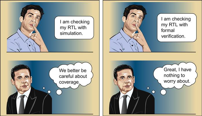
Thus we see that while FV engines are providing mathematical certainty in the domain of their analysis, there are many opportunities for users to provide erroneous input or specifications to the tools. This is not unique to formal methods, of course—this is true of nearly any type of verification method. The danger, however, is that the expectations are higher for FV: many managers know very little of the technical details, but have absorbed the meme that FV means mathematical certainty, as illustrated in Figure 9.1.
To clarify, we are not retreating from the main point of this book: FV methods are a very powerful and accurate means of design verification, and in many cases exponentially more effective and cost-efficient than simulation-based approaches. But we need to be careful to realize that FV is run by actual human beings, and thus is not exempt from the fact that it is possible to make mistakes. The most dangerous types of mistakes are what is known as false positives, where a design is reported correct but later found to contain a bug. When managers who expect that their design has been mathematically proven with formal certainty suddenly get reports of a bug in the “proven” products, they tend to be extremely unhappy. These are often a consequence of overconstraint, where user assumptions or directives prevent the tool from considering all legal behaviors.
We should also mention that another class of errors, false negatives, is common with FV tools. As we have seen many times in previous chapters, false negatives are an expected part of the verification process. Initial FV runs almost never include all the assumptions needed, so most FV engineers spend a large proportion of their time examining waveforms resulting from false negatives, figuring out why they are not really errors, and adding the proper assumptions or tool constraints. False negatives are significantly less dangerous than false positives, since they may result in extra engineering time, but will not lead to a buggy design being labeled correct. They are most often the result of underconstraint, where the tool is considering behaviors that should not be in the verification space.
Thus, false positives are the more critical concern when talking about ways FV might go wrong. We need to be careful to understand potential causes of these false positives and understand what we can do to prevent them. The best way to illustrate this is by looking at a set of real-life cases. So in this chapter, our discussion will focus on a number of examples where we or our colleagues have seen false positives: cases where a design was considered formally proven or “clean” at some point, and later found to contain a bug that was missed in the initial verification effort. Naturally, we have had to abstract many details of these examples, for space, simplicity, and readability, but you can be confident that anything you read in this chapter was based on actual FV work that took place at Intel. Based on these observations of real cases, we will then discuss what actions should be taken to prevent many classes of false positives.
Misuse of the SVA Language
One simple type of false positive can arise from the misunderstanding of SystemVerilog or the SVA assertion language. Some of these examples will likely seem silly or trivial on first reading, but remember that these are all based on real cases we have seen in practice.
The Missing Semicolon
Yes, you read that section title correctly: the first case we discuss is that simple, just one missing semicolon. Most people would probably think that missing semicolons would always be caught by the compiler, so why even worry about such cases? But in fact, the SVA language does provide the ability for a subtle case of a missing semicolon to effectively negate an assertion, causing an FPV proof to be skipped on a real design project.
To see how this happened, look at this code fragment:
assert property (foo)
assert property (bar) else $error(“Bar problem.”);
You have probably spotted a few oddities of the code above. First, the assertions are not labeled: remember that an SVA assertion starts with a label: before the assert keyword. However, labels are optional in SVA, so that alone is not technically a problem.
The real issue is: how is an SVA assertion terminated? The full SVA assertion syntax looks basically like this:
[<label>:] assert property (<prop>) [<pass_action>] [else <fail_action>];
In other words, after the assertion’s property expression, there are two optional action blocks: the pass_action, a SystemVerilog command to execute when the assertion passes, and a fail action, which is executed when the assertion fails. The semicolon marks the end of all action blocks.
This means that if an assertion is missing a semicolon, the next SystemVerilog statement to appear is considered its pass action—even if that statement is another assertion. So, for the first assertion above, we have:
The second assertion has become the pass action of the first one! In simulation, this might be okay, since whenever the first assertion passes, the next assertion is checked as its pass action. But FPV tools typically ignore the action blocks, which were mainly designed for use in simulation. This led to a real issue on a major design project at Intel, where a validation engineer discovered at a late stage that an assertion was being ignored in FV. It took some staring at the code with language experts to finally identify the issue.
Assertion at Both Clock Edges
An even more subtle case than an assertion being ignored is the case when an assertion exists, but is timed differently than the user expects. Look at the following assertion, intended to indicate that whenever a request signal rises, it is held for at least six cycles:
hold_request: assert property (@(clk1))
$rose(req) |=> ##6 (!$fell(req));
Have you spotted the subtle error here? Rather than specifying an edge of the clock, the clocking argument to the assertion just specifies a plain clock signal. Instead of @(clk1), the assertion should have used @(posedge clk1). As we saw in Chapter 3, in such a case the assertion is sensitive to both positive and negative edges of the clock. For simple Boolean assertions, being sensitive to both edges just results in extra checking, so is ultimately harmless, other than a slight performance cost. However, when there are repetitions or delays, as in the ##6 delay operator, this is much more serious: the count is effectively half of what the user intended, counting six phases, which are equivalent to three cycles.
This type of issue is especially insidious because the assertion will still be actively checked, and might even catch some real bugs. For example, if the request falls after only one cycle, or two phases, the assertion above will successfully catch the issue. In the real-life case where we encountered this situation, the user was especially confused because he had caught real errors when running FPV with this assertion, yet a simulation run late in the project reported that they had found an error, using an independent checker, where a request disappeared after five instead of six cycles. Again, it took a careful review of the code to properly identify this issue.
Short-Circuited Function with Assertion
Another subtle case involves assertions that may actually never get checked at all. It can occur when an assertion is placed inside a function, and some calls to that function are inside complex logic expressions. Look at this example code fragment:
function bit legal_state(
bit [0:3] current, bit valid;
bit_ok: assert #0 (!valid || (current != '0));
legal_state = valid && $onehot(current);
endfunction
. . .
always_comb begin
if (status || legal_state(valid, state)) . . .
Since a procedural if inside an always_comb is executed every cycle by definition, the author of this code thought he could be confident that the assertion bit_ok would always be checked. But this was incorrect, due to a clever feature of the SystemVerilog language known as short-circuiting.
The idea of short-circuiting is to leverage the fact that in certain types of logical expressions, you can figure out the ultimate result without examining all the terms. In particular, anything ANDed with a 0 will result in a 0, and anything ORed with a 1 will result in a 1. Thus, if you are analyzing an OR expression, you can finish as soon as you have determined that some term is a 1. Like the C programming language, SystemVerilog explicitly specifies this in the Language Reference Manual (LRM), stating that if the first term of an OR is 1 or the first term of an AND is 0, the remaining terms of the expression should not be evaluated.
In the example above, we see that status is ORed with the call to legal_state. This means that if status==1, tools are not expected to evaluate the function call—and as a result, assertions inside that function are not evaluated in such cases. This is another issue that may be deceptive to users, because they will likely see some cases, cases where status==0, in which the assertion is functioning correctly and can even detect bugs. But, as some unfortunate Intel users discovered the hard way through bug escapes, the assertion is effectively ignored by EDA tools when status==1.
Once understood, this issue can be resolved fairly easily. The simplest method is to place the function-containing argument first in the expression. Be careful if using this solution though: if you have multiple function-containing terms, you may need to break down the expression into several intermediate subexpression assignments to ensure all terms are evaluated every cycle.
Subtle Effects of Signal Sampling
This is another very tricky SVA issue, a case where an assertion was apparently generating an incorrect result that took many hours of debug to finally understand. This issue results from the sampling behavior defined for assertion variables. In the following code fragment, look closely at the signals passed in to the assertion:
input logic[31:0] index;
. . .
current_pos_stable: assert property ($stable(req[index]));
At first glance, this seems like a relatively simple property. We have some vector req, and wish to ensure that whichever position in the vector is currently selected by index has been stable for at least one cycle. But what values are being used for req and index?
Remember that concurrent assertions and sampled value functions like $stable always use the sampled value of each variable, in effect the final value of the variable from the end of the previous time step. The trick here is to recognize that there are two sampled values in the property expression above: req and index. The $stable function uses the last value of each of them for its check: so if index just changed, it will actually compare the current value in the current position of req to the last cycle’s value in a different position! The waveform in Figure 9.2 illustrates an example of this situation causing a false negative, where each element of the vector is stable, but a moving index causes the expression $stable(req[index]) to be unstable.

In real life, this situation is dangerous, in that it can generate both unexpected false negatives and unexpected false positives. And once again, this is an example where in many cases, those where the index is not moving, the assertion can seem to be working fine, and successfully help to detect many real RTL bugs. The fact that some subset of cases is not being correctly checked may easily be missed.
This one is also a little trickier to solve than some of the other cases we have mentioned. When we faced this issue, our key insight was to realize that we really want the index to be constant for each comparison, even though we wanted the req vector to be sampled as normal. We were then able to solve it by using a generate loop to define the index as a compile-time constant, creating a family of assertions checking that for each constant index, if it happens to be currently active, the stability condition is met.
generate for (genvar i = min; i < max; i++) begin
current_pos_stable: assert property ( (i == index) |->
$stable(req[i]));
end
Liveness Properties that are Not Alive
The final SVA issue we describe relates to an advanced feature of FPV, the ability to analyze “liveness” properties on traces of potentially unbounded length. For example, as we have seen in earlier chapters, this assertion states that a request will eventually get a response:
response_good: assert property (
request |-> s_eventually(response));
The s_ before the eventually indicates that it is a strong property: even if it has no finite counterexamples, it can be falsified by an infinite trace that enters a loop in which the awaited condition never happens. This contrasts with weak properties, which can only be falsified by a finite counterexample, and are considered true if no such finite counterexample exists.
In SVA, properties are weak by default, unless an explicitly strong operator is used. This means that the property below, even though it might seem conceptually similar to the one above, can never fail in FPV; when looking at any finite “counterexample,” you cannot be sure whether the response would have arrived a few cycles after it ended:
response_weak: assert property (
request |-> ##[1:$](response));
Unfortunately, the concept of strong and weak properties was not clearly defined in the 2005 LRM. These ideas and related operators such as s_eventually were introduced in the 2009 revision. Before that, properties like response_weak above were the only practical way to express liveness, so most FPV tools built for SVA 2005 were designed to treat ##[1:$] properties as implicitly strong.
This created some pain when some Intel projects upgraded from SVA-2005-compliant to SVA-2009-compliant tools. When initially ported, all of the liveness properties written in the ##[1:$] form seemed fine—they had passed on the existing (already verified) models before and after the upgrade, so initially we thought that our FPV runs were properly checking them, and happily moved forward with the changes.
It was only after a user made a change that they knew should invalidate some liveness properties, and became confused when they all still passed, that we realized something incorrect was happening. In effect, all our liveness properties were unfalsifiable, since they were considered weak by default under the new standard. Thus, ever since the upgrade, none of the liveness proofs on properties written in the old 2005 style were valid. We had to modify our code to fix all such cases, or get our tool vendors to slightly violate the LRM and treat 2005-style liveness assertions as strong.
Preventing SVA-Related False Positives
Our best advice for preventing these kinds of issues is probably something you have heard in other contexts as well: run good lint checks on your RTL. Linting, the process of running a software tool that does structural checking on a piece of RTL to find common cases of legal code with unintended behavior, has become very standard and mature in the industry. If you are a serious, well-disciplined designer (very likely, given that you had the wisdom to decide to read this book), you need to be running regular lint checks on any RTL code you develop.
If you are relying on other team members or many layers of scripts to get your RTL lint checks done, be careful to double-check that your assertion code is included in the linting. Due to early lint tools that generated some bogus warnings on SVA assertions, we have seen many cases of projects that show excellent discipline in RTL linting, but exclude SVA code from the process completely. If your coworkers are nervous about enabling linting for SVAs, just show them the examples above in this section, and there is a good chance they will reconsider.
One other critical factor in linting is to make sure you have a good set of lint rules implemented. The cases we have discussed in this section inspire rules like the following:
• Flag any assertion that exists entirely inside another assertion’s action block.
• Flag any assertion that is active at both clock edges.
• Flag any assertion-containing function that is invoked in a short-circuitable position of a logical expression.
• Flag any case where a sampled variable is used as a vector index in an assertion or sampled value function.
• Flag any properties that seem to be aimed at liveness and are weak due to being written in the SVA 2005 style.
Keep in mind that, due to lack of space, the cases in this section were just a few examples; for a more complete set of SVA-related lint rules, see [Bis12] and talk to your EDA vendor to make sure a good set of SVA lint rules are implemented.
We should also mention, however, that manual review is always a good supplement to lint checks. While linting can detect a wide variety of issues as we mention above, we have seen that the SVA language does contain many pitfalls and opportunities to write assertions that do not say exactly what the author intended. Thus, we suggest that every unit also plan assertion reviews with an SVA expert before the RTL design is closed.
Vacuity Issues
As we have discussed throughout this book, one important consideration when doing FV is vacuity: the idea that you may have unintentionally overconstrained the environment. This would mean that important behaviors in the verification space are ruled out by your assumptions or other parameters of your proof setup. In the worst case, if you create an assumption that defines a globally false condition, such as (1==0), all possible inputs may be ruled out, and all assertions are trivially considered true due to the absence of any legal inputs at all. When this happens, your FV proofs will be reported as passing—but will potentially be overlooking key bugs.
Misleading Cover Point with Bad Reset
The next case we discuss is another seemingly trivial error, but one that can have consequences that are a bit subtle if you are not careful. Remember that one important technique we use to sanity-check our formal environments is proving cover points. These show that under our current set of assumptions and settings, we are able to replicate interesting behaviors in our design.
An important aspect of cover points that requires extra care is the reset condition. Remember that during the reset stage of a design, it is often possible for many internal elements to attain transitory “garbage” values that do not represent actual computation. This is why the SVA language provides the reset feature (disable iff) for assertion statements, to shut them off during reset. For an ordinary assertion, if you accidentally provide the wrong reset argument, you will quickly catch this during simulation or formal analysis, as bogus failures are reported during reset. But what happens if the reset argument to a cover point is wrong?
A cover point with an incorrect reset may be reported as covered, due to the garbage values see during reset—but it is entirely possible that the cover point is not reachable outside reset, and this coverage report is hiding a real vacuity issue. Here is an example cover point, based on a real case from an Intel design:
c1: cover property (disable iff (interface_active_nn)
(data_bus != 64’b0));
This cover point is checking that a data bus is capable of attaining a nonzero value, a good type of check to include in any formal environment. The reset signal name interface_active_nn on this design follows a convention that signals ending in nn are active on 0 values instead of 1, but this slipped the mind of the cover point author: the disable term should really be based on !interface_active_nn. As a result, instead of being shut off when the interface was inactive, this cover property checked the data bus only when the interface was inactive. This resulted in an incorrect report that the condition was covered, when in fact some bad FPV tool directives were preventing any nonzero data in cases where the interface was active. The issue was discovered when bugs in the “proven” part of the design were later reported from simulation.
The reset conditions are a fertile ground for generating broken verification environments. The above example is just one of many cases we have observed where some portion of a design was deactivated due to expecting a reset of opposite polarity. This can be especially dangerous in designs with multiple reset signals, where it is possible that some subset are correct, creating the illusion of some nontrivial activity, while others are wrong.
Another critical thing to watch for is cases where an FPV environment “cheats” to simplify the reset process. Many tools have an option available to look for any flops that do not have a determined value after reset, and automatically set such flops to 0 (or to 1). This can often save time in early stages of setting up FPV on blocks with complex reset. But this can also hide a class of bugs, since if you have flops with an indeterminate starting state, you need to make sure that your model behaves correctly regardless of what values they assume. This has also happened to us in real examples.
Proven Memory Controller that Failed Simulation
The next example we discuss shows a case where the set of assumptions and cover points provided an interesting and powerful FPV environment—but one crucial requirement was not properly communicated from a neighboring unit.
In one of our chipset designs, we verified a number of properties of a memory controller block. This was a block that received requests, related to performing some operation at a particular memory address, and processed them according to the opcode passed in, as illustrated in Figure 9.3.
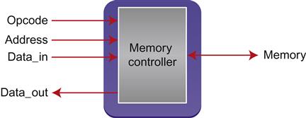
When initially proving the assertions on this design, the validation engineers encountered a number of counterexamples with a common cause: an opcode and address would specify a multicycle operation, but before the operation would complete, the address on the address bus would change. After finding this situation and discussing over the course of several meetings, the engineers involved in this effort agreed that changing the address of a pending request would be an absurd way to use the memory controller, and thus could be ruled out by an assumption. Once this assumption was added, the properties were fully verified, finding a few RTL bugs along the way and resulting in completing the FPV effort with high confidence.
However, as it turned out, the assumption that the address bus would not change during an operation was incorrect. This requirement had not been clearly communicated to all designers, and some of the RTL had been written with the implicit idea that after the cycle when a request was made, the controller would have already captured the address in local memory, and thus not care if garbage values appeared on the address bus while the operation was in progress. Thus, the unit supplying the inputs to this model really would change the address of pending requests, rendering some of the initial FPV proofs invalid. In this case, the assumptions ruling out these inputs had actually ruled out a part of the real problem space, as currently understood by the neighboring unit’s designer.
Fortunately, this was discovered before tapeout: the FPV assumptions were included in the full-chip simulation regressions, and these regressions detected the failing assumptions, alerting the validation team of this disconnect in requirements. This also uncovered a real RTL bug where if the address bus changed when a request was pending, the design would behave incorrectly. Both the RTL code and FPV environment needed to be fixed after this failure was observed.
In general, this issue points to the importance of the assume-guarantee philosophy behind FV. Whenever using assumptions in FV, you should always have a good understanding of how their correctness is verified, whether through FV on an adjacent unit, extensive simulation, or careful manual review.
Contradiction Between Assumption and Constraint
The next case we discuss was one of the most disastrous ones in this chapter: it is a case where an Intel validation team, including one of the authors, reported that a design was FEV-clean for tapeout, indicating that we were confident that we had formally proven the RTL design was equivalent to the schematic netlist. However, when the chip came back from the fab and we began testing it, we discovered that the first stepping was totally dead—and this was due to a bug that should have been found by FEV.
After many weeks of intense debugging, we figured out that the FEV environment was vacuous: the proof space contained inherent contradictions. Remember that any formal tool is analyzing the space of legal signal values, under the current set of assumptions and tool constraints. If this space is completely empty—that is, there are no legal sets of inputs to the current design—then the formal tool can report a trivial “success,” since no set of inputs can violate the conditions being checked. Most modern formal tools report an error if the proof space is null, but this feature had not yet been implemented in the generation of FEV tools we were using on that project.
However, there was still a bit of a mystery: how could this happen when we were running nightly simulations? All our assumptions were being checked in simulation as well as FV, so shouldn’t some of the contradicting assumptions have generated simulation errors? The subtlety here was that there are various kinds of tool directives that implicitly create assumptions. In particular, as we discussed in Chapter 8, FEV environments use key point mappings to show how the two models are connected. Many of these mappings can create implicit assumptions as well. For example, look at the one-many mapping:
sig -> sig_dup_1 sig_dup_2
This represents a case where a single flop in the RTL design, sig, was replicated twice in the schematics. This is a common situation for timing reasons; while it makes sense logically to think of a single signal sig in the RTL, physically it needs two replicated versions to drive different parts of the die. In this case, we are also implicitly creating an assumption equivalent to
implicit_assume: assume property (sig_dup_1==sig_dup_2);
In other words, any time we have a one-many mapping, we are implicitly telling the tool to assume that all the signals on the right-hand side have the same value.
In the FEV failure we are currently discussing, one mapping looked like this:
myflop -> myflop_dup_1 myflop_inv_1
This represents a case where a single flop in the RTL design, myflop, was replicated twice in the schematics. This is a common situation for timing reasons; often a high-speed circuit can be implemented more efficiently if a flop is replicated twice to drive it signal to diverse locations on the die. In this case, one of the replicated flops is logically inverted, as indicated by the _inv_ in its name. Usually in such cases we expect an inverse mapping:
myflop -> myflop_dup_1 ~myflop_inv_1
The FEV owner happened to omit the ~ sign before the inverted flop. This created a major issue because without the inversion, this mapping was creating an implicit equivalence between myflop_dup_1 and myflop_inv_1. But elsewhere in the design, there was a direct assumption that the two signals myflop_dup_1 and myflop_inv_1 were inverse of each other:
a1: assume property (myflop_dup_1 == ~myflop_inv_1);
Together, the broken mapping and the assumption above told the FEV tool that the only legal cases were ones where myflop_dup_1 was both equal to and the inverse of myflop_inv_1—so the set of legal inputs became the null set. The verification was then reported as passing, because no set of legal inputs could violate the equivalence property. This passing status was vacuous, actually checking nothing, but at the time we did not have an FEV tool version that automatically reported vacuousness. A last-minute manual RTL change had been made, so there really were nonequivalent key points, which went undetected before tapeout.
Most modern FEV tools have features to automatically report this kind of totally vacuous proof, but we still need to be careful of the dangers of partially vacuous proofs, where accidental overconstraints rule out large parts of the desired behavior space.
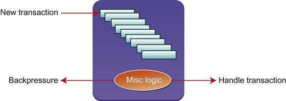
The Queue that Never Fills, Because it Never Starts
Our next example comes from a chipset interface design where a set of incoming transaction requests is placed in a queue, which has a limited size. Periodically the control logic removes the next transaction from the queue for processing. However, the time taken per transaction can vary, so there is a danger of the queue overflowing when too many messages arrive at the wrong time. When the queue is almost full, it sends a backpressure signal to indicate that no more transactions should be sent.
The design constraints for this interface were very tight: the designer wanted to ensure that the queue would never overflow, but also did not want to send out an overly cautious backpressure signal that would stop traffic too early and reduce effective bandwidth. She implemented some backpressure functionality that seemed to work correctly in all the simulation tests she tried, but was still nervous that the design might be failing to send backpressure in some rare cases that could generate an overflow. Thus, she asked for help from the FPV team. Figure 9.4 illustrates the verification challenge at a high level.
When setting up the design for FPV, the validator created a good set of assertions to prevent queue overflow and added numerous assumptions related to the legal opcodes and other control signals for the transactions. After debugging some initial problems with verification environment and some other constraints, the assertions were all proven true in FPV.
However, the designer was initially skeptical based on how (apparently) easy the process had been and requested some more solid evidence that the FPV environment was working properly. The validator responded by adding various cover points, including ones to observe completed transactions. It was a good thing they did this—because it turned out that no completed transactions were possible! Due to a simple flaw in an assumption, requiring that an opcode be illegal instead of requiring that an opcode be legal, all ordinary transactions were ruled out. The flaw was similar to the following:
// Variable transaction_check is 1 if transaction is BAD
assign transaction_check =
((opcode != LEGAL1) && (opcode ==LEGAL2) . . .)
// Assertion missing a ~
a1: assert property (transaction_check);
Fortunately, once the cover point failure was discovered, the designer and validator were able to identify the flawed assumption and fix it. After this was done, a rare overflow condition was discovered, and the designer realized that the backpressure signal needed to be generated with slightly more pessimism. After this RTL fix, she was able to prove the design correct with confidence, observing that all the cover points were covered and the assertion proofs passed.
As you have read in earlier chapters, we always recommend that you include a good set of cover points in your FPV efforts, just as the designer and validator did in this example, to help detect and correct overconstraint.
Preventing Vacuity: Tool and User Responsibility
As we have seen in the examples in this section, we must constantly think about potential vacuity issues when doing FV. A naïve view of FV is that it is solely about proving that incorrect behaviors never occur, and once you have done that, you have full confidence in your verification. However, an equally important part of the process is to verify that, in your current FV environment, typical correct behaviors are included in the analysis.
The techniques that we mentioned in the previous section—linting and manual reviews—are a good start. They can detect a wide variety of situations where an incorrectly written assertion is leaving a hole in the verification. The case of the cover point with bad reset polarity could have been discovered earlier if these methods had been used correctly. But these are just a beginning; there are several more powerful methods that should also be used to prevent vacuity.
The most commonly used vacuity prevention method is to include FV assertions and assumptions in a simulation environment. We are not suggesting that you do full simulation-based verification on each unit that replicates your FPV effort. But in most real-life cases, full-chip simulation needs to be run anyway, to get a basic confidence in full-chip integration and flows, while FV is run at lower levels or on partial models. While it covers a much smaller space than FV, simulation tends to actively drive values based on real expected execution flows, and so it can often uncover flawed assumptions. Such a simulation revealed the bad memory controller assumption in our second example above. Thus, you should include your FV assertions and assumptions in simulation environments whenever possible.
Due to increasing awareness of vacuity issues, many EDA FV tools include built-in vacuity detection. Tools can now detect cases where a set of contradicting assumptions rules out the entire verification space, as in the example above where we had a contradiction between an assumption and an FEV mapping constraint. Most FPV tools also offer “trigger checks,” automatic cover points to detect at the individual assertion level when an assertion precondition is not met. Some formal tools also offer coverage checking features, where they can try to identify lines, branch points, or other important parts of RTL code that are and are not covered in the current FV environment. You should be sure to turn on these features if available in your current tools.
You need to be careful, however, not to be overly confident in the automated checks of your tools. For example, automated vacuity checking may report that the proof space is not empty, while large classes of interesting traffic are being ruled out. This is what happened in our example above with the queue that could never fill. The proof space was not fully vacuous, since the design could participate in scan protocols, power down, and other secondary tasks. Yet the most important part of the design, the processing of transactions, was effectively disabled by broken assumptions.
The best way to discover this kind of situation is by adding cover points: try to think of typical good traffic for a design, and cover examples of each common flow. When these are reported as covered, you can look at the resulting waveforms and gain confidence that your expected behaviors really are possible under your current formal constraints. You may be getting a sense of déjà vu by now, since we have emphasized this point at so many places in the book—but that is because it is so important. In any FV effort, creating a good set of cover points is critical.
A final piece of advice for preventing vacuity is to always be conscious of the reset sequence you are using. Start by reviewing the polarity of every reset signal you use, and make sure they are correct. You should also try to make your reset as general as possible: do not force starting values of 0 or 1 on nodes that are truly not reset or you may risk hiding some real issues.
This advice may seem like somewhat of a contradiction from some earlier chapters, where we suggested the use of intentional overconstraint to reduce complexity or stage the verification process. Those suggestions still apply though; here we are pointing out the potential dangers that can result if you do not follow them carefully. Make sure you are fully aware of any intentional overconstraints, or reset and initialization conditions that are not fully general, and can justify and document why these do not create a gap in your verification process.
Implicit or Unstated Assumptions
When thinking about vacuity issues, as we discussed in the previous section, each user tends to focus on the set of assumptions and tool constraints that they created as part of their formal environment. But what if something inherent to the environment is quietly creating assumptions or constraints on its own? Often it is possible that tools or libraries come with their own set of implicit constraints, and the user needs to be careful that they are using the tools properly in their current context. We have seen some situations where these implicit assumptions have caused problems that were caught very late in a project.
Libraries with Schematic Assumptions
As we mentioned in Chapter 8, schematic netlists are often built based on standard cells, basic logic elements such as AND gates, OR gates, and muxes, that have been pre-designed at the transistor level and can be instantiated to implement the desired logic. These libraries are pre-verified: if a cell claims to be an AND gate, an FEV tool can accept that as an axiom, rather than having to go through the compute-intensive process of doing every proof at the transistor level. Thus, they are a key factor in making FEV practical and commonplace.
However, in some cases a library cell may include optimization that depends on some assumptions on their inputs. Figure 9.5 shows an example of such a case.
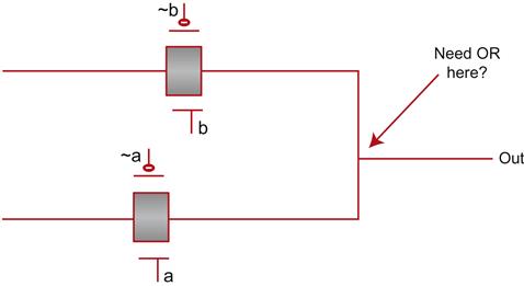
This is a simple selector that drives the upper value to out iff signal b is high, and drives the lower signal to out iff signal a is high. But if you remember your introductory electrical engineering class, you can probably spot a few problems in this design. What if neither a nor b is high? In that case, out is a floating node, very undesirable in most cases. And even worse, if both are high, then the two input wires are shorted together. On the other hand, this cell is much better for area and performance than the “safe” version would be, since that would require many more transistors. If we can guarantee at all times that precisely one of these values is 1 and the other is 0, this cell should be acceptable in practice.
Thus, a library may be delivered with some required assumptions for certain cells. Users of such a library are required to guarantee that these assumptions will be met if these cells are used. Thus, in the FEV process for designs containing such libraries, an extra step is needed: schematic assumption verification. This is essentially a miniature FPV run focused on the set of properties in the library. If this is omitted, the library cannot be trusted to deliver the claimed functionality.
The lack of understanding of this requirement is what led to another case of dead silicon on an Intel design. An engineer responsible for a late change on a project reran the FEV flow to check his edits. He did not understand the purpose of the schematic assumption verification step, and looking up the documentation, he read that it was a form of FPV. Since FPV was not listed in the required tapeout checklist for this particular block (the main validation strategy was simulation), he marked his FEV run as clean with that step disabled.
As a result, the design was not using its library cells safely, and the initial silicon came back dead. The omitted schematic assumption step was discovered when FEV experts re-examined all the tapeout flows as part of the debug process.
Expectations for Multiply-Driven Signals
Another common case that can create confusion is when the tool makes some implicit assumption common to the industry and misinterprets the intention of a design. An example of this situation is the case of RTL signals with more than one driver. How should such a signal be handled? It turns out that there is a common convention, used by many industry synthesis and FEV tools, that a multiply-driven RTL signal should be handled as a “wired AND.” The result should be interpreted as the AND of all the drivers, and the synthesis tool should generate a circuit where the multiple drivers are combined with an AND to generate the overall value. This interpretation is the default in many tools.
On one recent Intel design, a late stage inspection of the schematic revealed that a connection at the top level was different than what the designer expected. On closer examination, we discovered that one of the wires involved had been declared as an “inout” at a cluster interface where logically it should have been an input. This meant that the top-level net that was driving it became multiply-driven, as it could get values from either its true driver or the inout signal. The synthesis tool had then synthesized AND logic for this net. The design had passed FEV, despite this difference between the RTL and netlist, because our FEV tool defaulted to treating multiply-driven signals as wired AND gates.
Once the issue was discovered, we were able to fix the problem in the netlist. We also changed the settings of our FEV tool to treat multiple driver situations more conservatively: it would examine every driver and make sure that for each node, the precise set of drivers matched between the RTL and netlist. This would automatically uncover cases where such a net is synthesized into a wired gate by the synthesis tool. We were then able to rerun FEV and prove that, under our now-stronger definition of equivalence, there were no further errors.
Unreachable Logic Elements: Needed or Not?
Another area where many FEV tools have a default view that can cause problems is in the issue of “unreachable” logic elements. Remember that, as we discussed in Chapter 8, many FEV tools simplify the equivalence problem by breaking up the designs at internal flops and verifying the equivalence of each of those flops between the designs. If a subset of flops targeted for verification in one design do not have a corresponding element in the other, it is reported as a mismatch in most cases.
However, a common exception to this methodology is what is known as an unreachable point. An unreachable point is a node in the design that cannot affect any output. These are most often due to some subset of the logic functionality that has been logically tied off, perhaps the implementation of some mode from a previous design that no longer exists. Another case is totally disconnected logic elements. These may arise from the insertion of “bonus cells,” extra logic that does nothing in the current design, but is placed on the chip in areas with extra open space, in case a late logic fix is needed and the design team does not want to redo the entire layout. Figure 9.6 illustrates the concept of reachable and unreachable points.
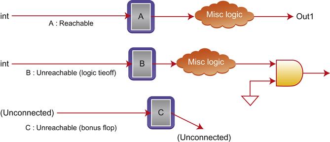
How should FEV tools handle unreachable points? Intuitively, we might expect that all such points should be reported, and the users could double-check to make sure the list is reasonable, identifying any that look suspicious. If comparing RTL to schematics, and some known modes were tied off or disabled in the design, some unreachable points could be very reasonable. But if comparing a schematic design before and after a small change, we would expect unreachable points to be very rare, and each one should be scrutinized very carefully.
However, as it turned out, one of our FEV tools had a default setting that would report unreachable points due to tied-off logic, but silently ignore completely disconnected nodes. In one of our chipset designs a few years ago, the schematics had been fully designed, gone through several validation flows, and was in a stage where backend designers were making minor schematic changes to optimize timing and area. Each designer who had touched the schematics had diligently run FEV to compare the models before and after their changes and make sure their edits were safe. But one of them carefully did a last-minute visual inspection of the layout, and discovered a surprising open area with no bonus cells.
It turned out that one of the late edits had been done with a script that accidentally deleted a large class of bonus cells. All the FEV flows had passed, because (at the time) none of the team was aware that the tool’s default setting ignored disconnected cells when checking equivalence. This was a lucky find: some later post-silicon fixes would have been significantly more expensive if the team had taped out without these bonus cells. Once the team determined the root cause of the issue and realized the mistake in the FEV settings, they were able to fix them so future edits would not face this risk.
Preventing Misunderstandings
The kind of issues we discuss in this section, where a user misunderstands the underlying behavior of formal tools and libraries, are among the hardest ones to detect and prevent. However, there are a few good strategies that can be utilized to minimize these issues.
You should be sure to understand the validation expectations of any external components or IP used in your design and delivered by another team. If someone else is providing a library of cells used in your RTL-netlist FEV runs, make sure to check for any requirements related to schematic assumption checking. Similarly, if integrating an externally provided IP or similar module and trusting its functionality rather than re-verifying it, make sure you verify that your design complies with its interface requirements.
In addition, review all tool control files with an expert in the relevant tool. This is a little different from our suggestion a few sections back about assertion reviews: here the required expertise is not in the content of the design itself, but in the tools used with the design. In all of the examples above, an expert with a proper understanding of the tools could have spotted and prevented the issues. Review by an expert can often help reveal potential issues and unexpected implicit requirements.
One other strategy is to be careful about the settings in any tool you use. There are usually a variety of options to control how the verification environment will behave, and often there are more forgiving and more conservative ways to set the options. If you do not fully understand some verification step, like the schematic assumption step in one of the cases above, the conservative choice is to turn it on by default unless you are sure it can be safely turned off. As another example, options that allow weaker checking of some design construct, such as treating multiply-driven nets as wired AND gates, or ignoring some classes of unreachable cells, are inherently dangerous and you should be careful about them. Where you have a choice, try to choose the more conservative option, so you do not gloss over any real errors. You need to be careful here, as in some cases your tool may have a weaker default that matches common industry practice.
Division of Labor
The final class of false positive issues we discuss relates to cases where we divide a problem into subproblems. It is often the case that we cannot run our FV task on a large design all at once; as we have seen in our discussions of case-splitting strategies in earlier chapters, subdividing the problem is often a critical enabler for FV. We also have cases where a portion of a design, such as an analog block or a complex floating point operation, is beyond the domain of our current tools and must be verified separately through other means. But whenever we subdivide the problem, we need to make sure that the sum total of our verification processes verifies all parts of the design.
Loss of Glue Logic
As we have mentioned above, it is very common for an analog block to be blackboxed for the purpose of FV. In one of our test-chip designs, we had such a case, where the FEV owner was responsible for verifying that the RTL and schematics matched from the top level down to the boundary of an analog block, while the analog block owner was responsible for a separate (simulation-based) verification process to ensure the correctness of that block’s schematic netlist.
The actual instantiation of the analog block was similar to the illustration in Figure 9.7, with a small amount of glue logic connecting the true analog logic to the design.
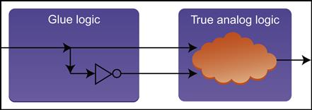
This raises an interesting question: which team is responsible for verifying the RTL-schematic equivalence of the glue logic? In this case, there was a bit of miscommunication. The analog design owner thought it was outside his domain of responsibility, since the glue logic looked like any other synthesizable block, just a small set of gates easily analyzable by a standard FEV tool. But from the point of view of the synthesis FEV owner, the glue logic was part of the analog block, so his verification blackboxed at the level of the outer boundary in Figure 9.7. As a result, nobody considered themselves responsible for verifying the glue logic. Despite the fact that it was a relatively trivial handful of gates, it was off by one inversion, causing incorrect functionality for the first stepping.
This is an error that could have been easily detected during pre-silicon FEV, if only the glue logic had been correctly included.
Case-Splitting with Missing Cases
Another common way that a FV task can be subdivided for complexity is through case-splitting. It is often convenient to subdivide for different modes, especially in a model that can be used in several different modes that are not expected to change dynamically. One example of this is in a chipset design where we were supporting the PCI Express (PCIE) protocol, a popular bus interface protocol that has several modes that support varying degrees of parallel traffic, known as x4, x8, and x16 mode.
In the PCIE block of one chipset design a few years ago, the designer was worried that some complex changes that had recently been made to improve timing and area might have caused bugs in the functionality. Thus, he asked an FPV expert to help set up a verification environment and check that the block would still work as expected. When the validation requirements were originally described, once again there was a slight miscommunication issue: “We changed functionality for the x8 mode” was interpreted to mean, “We only need to verify the x8 mode.” The FPV expert set up the initial verification environment, helped prove and debug numerous assertions about the design’s functionality, and even found some very interesting RTL bugs along the way. Eventually he reported that the verification was complete, as all the assertions were proven.
During a review of the “complete” verification, it was discovered that the FPV environment only covered the x8 mode. The designer then explained that while this was where the most interesting changes were, the logic for all the modes was intertwined in many places, and verification was still required for the x4 and x16 modes in addition. Thus, the verification run was not as complete as originally thought and required several more weeks of work, during which one additional bug was found, before being truly finished.
Another very similar example came from a case where we were verifying an arithmetic block, with a 6-bit exponent. To simplify the problem, it was split into two cases: one where the value of the exponent ranged between 0 and 31, and the other where it ranged from 33 to 64. As the astute reader may have already noticed, the validator forgot the critical value of 32, which turned out to be especially risky (being a power of 2) and was the one case with an implementation bug. The bug was discovered much later than desired.
Undoing Temporary Hacks
An additional hazard related to division of labor can occur when one part of the team believes they own a piece of validation collateral, and thus can freely hack it to make things convenient for various EDA tools. By a “hack,” we mean a change to the collateral files that may be logically unsound, but due to tool quirks or bugs, makes some part of the verification process more convenient. In an ideal world, we would never have to do such things to make our tools happy. But sadly, most VLSI design today occurs in the real world rather than an ideal one.
In one of our chipset designs, some team members used a new timing tool and found that it had a problem with a bunch of our library cells. We had some cells in our library that consisted of a pair of back-to-back flops, a common situation for clock domain crossing synchronization. This new timing tool, due to a software bug, had a problem handling these cases. The timing engineers noticed that the library cells were available in two formats: one was a proprietary format, intended mainly for timing tools, and the other was in standard Verilog. Thinking that they were the only users of the proprietary format, they hacked the files so each pair of flops was replaced by a single one. The modified files were then checked in to the repository for future use.
Unfortunately, the timing engineers’ assumption that the proprietary format was used only for timing was not quite correct. These files actually could optionally be used instead of Verilog by both synthesis and FEV tools, and the presence of the corrupted files led to numerous two-flop synchronizers throughout the design being quietly replaced with single flops during design and verification flows. Because synthesis and FEV both used the corrupted files, the problem was not detected until very late in the project. Fortunately, a manager questioned the use of the proprietary format for FEV, and the team decided that it was safest to base the equivalence checking on the Verilog representation. Once this was done, the true issue was discovered, and the design could be corrected before tapeout.
Safe Division of Labor
The issues discussed in this section are another set of cases where the human factor becomes critical. In most cases, there is no way a single person can fully verify a modern VLSI design; the verification problem must always be broken down into many subproblems, with the proper specialists and tools taking care of each part. However, we must always keep in mind that there should be someone on the team with a global view, someone who understands how the problem has been divided and is capable of spotting cases of a disconnect between owners of different portions of the verification. There should always be validation reviews at each major hierarchy and at the full-chip, including both the owners of the subproblems and a global validation owner who understands the big picture.
Aside from the understanding of the overall validation process, understanding the tools involved remains important for this set of issues as well. As we discussed in the previous section, tools have many individual quirks and hidden assumptions, and it is best to have someone with a good understanding of the tools involved participate in the reviews. The discovery of the issue of hacked cells that were fooling FEV and synthesis, for example, stemmed from a tool expert questioning the slightly dangerous use of poorly understood proprietary formats when running FEV. Thus, these issues provide yet another reason to pay attention to the tip in the previous subsection and try to always include a tool expert in validation reviews.
Summary
In this chapter we have explored various types of issues that have led to false positives in FV: cases where some type of FV flow was run, and at some point in the project, the design was labeled “proven” when there was actually something logically unsound about the verification. The worst cases of false positives led to the manufacturing of faulty chips, resulting in massive expense and costly delays to fix the designs and create new steppings.
The major classes of mistakes we observed that led to false positives included:
• Misuse of the SVA language. As we saw, there are numerous cases in which the details of SVA can be tricky. Issues ranging from a simple missing semicolon to complex sampling behavior can cause an SVA assertion check to differ in practice from the user intent. Any code where nontrivial SVA assertions are used should be subject to good linting and manual reviews.
• Vacuity issues. There are many ways that a significant part of the verification space may be eliminated from an FV process. It is critical to think about both cases of full vacuity, where the verification space is the null set, and partial vacuity, where there is an interesting verification space but important cases are ruled out. Tool features can be used to detect a subset of these problems, but these should always be supplemented with manual cover points, and with inclusion of FV assertions and assumptions in available simulation environments.
• Implicit or unstated tool assumptions. Many EDA tools have implicit defaults or assumptions based on the most common usage patterns in the industry, which may or may not apply to your particular case. You should carefully review your settings and run scripts with a tool expert, trying to err on the side of choosing more conservative options whenever you lack a detailed understanding of some part of the process.
• Division of labor. Due to the complexity of modern designs and the variety of validation problems, division of labor among teams and processes is usually unavoidable. But this type of division also creates the danger that some portion of the design or validation problem remains uncovered, because of miscommunication or misunderstandings among the subteams involved. You need to make sure someone on the team has a global view and is helping to review the various pieces of the validation process and to ensure that they all fit together correctly.
Again, while the discussions in this chapter reveal some subtle dangers where misuse of FV led to expensive rework, we do not want to scare you away from FV! Most of the false positive situations above actually have analogs in the simulation world; and in simulation, the problems are compounded by the fact that coverage of the validation space is so limited to start with. As you have learned by this point in the book, FV is a very powerful technique that leads to true coverage of your mathematical design space at levels that simulation engineers can only dream of. But with this great power comes great responsibility: to understand the limits of the FV process and to take whatever action we can to reduce the danger of missing potential issues. By understanding the cases discussed in this chapter and using them to inform your FV flows, you can formally verify your designs with even greater confidence.
Practical Tips from This Chapter
9.1 Always run lint checks on any RTL code you develop.
9.2 Double-check that SVA assertion code is included in your project’s lint processes.
9.3 Make sure that your project’s linting program includes a good set of SVA-related lint rules.
9.4 Review each unit’s assertions with an SVA expert before tapeout, to help identify cases where the assertion doesn’t quite say what the author intended.
9.5 Always include your FV assertions and assumptions in any available simulation environments.
9.6 Turn on any vacuity checking, trigger checking, and coverage check offered by your EDA tools, and look carefully at the results.
9.7 Always create a good set of cover points representing typical behaviors of your design, to help sanity-check the proof space of your FV environment.
9.8 Review the interface expectations of any externally provided libraries or IPs whose functionality you are trusting rather than re-verifying. Make sure your verification plan includes checks that you are complying with any documented requirements.
9.9 Before completing a project, review your FV environments and tool control files with an expert on the tools and libraries involved.
9.10 Double-check the polarity of all reset signals and make sure that their values in the FV environment match the design intent.
9.11 Make your reset sequences for FV as general as possible, not setting any signals that do not need to be set for correct FV proofs. Be especially careful of tool options that allow global setting of 0/1 on nonreset nodes.
9.12 Make sure you are fully aware of any intentional overconstraints, or reset and initialization conditions that are not fully general, and are used to stage the verification process or reduce complexity. Justify and document why these do not create a gap in your verification process.
9.13 Review options that your FV tool provides, and try to choose more conservative checks in preference to weaker ones, unless you have a strong understanding of why the weaker options are acceptable for your particular case.
9.14 Whenever a validation problem is subdivided among several owners, somebody should be responsible for understanding the global picture and should conduct reviews to make sure all the pieces fit together and every part of the divided problem is covered.