
4.5 Cross-buying
Cross-selling is the most common technique companies use to increase the repeat purchase incidence, quantity, and revenues to companies. After companies have built a certain level of loyalty with existing customers, these customers are more likely to cross-buy from the company. Verhoef and Donkers [5] studied the effect of acquisition channels on cross-buying. The acquisition channels examined included mass media, direct marketing, the Internet, personal selling, intermediaries, and word of mouth. For customers who were retained, cross-buying was coded as a binary variable. These authors modeled cross-buying in a probit model and acquisition channels were included as dummy variables.
4.5.1 Empirical Example: Cross-buying
Another key question we want to answer with regard to customer retention is whether we can determine which customers have the highest likelihood of cross-buying in multiple categories. To do this we first need to know which current customers actually purchased in multiple categories when they made a purchase. In the dataset provided for this chapter we have a variable Crossbuy which identifies how many categories of products a customer purchased in a given time period. We also provide a set of drivers which are likely to help explain a customer's decision to cross-buy. At the end of this example you should be able to do the following:
A B2C firm wants to understand which customers are most likely to cross-buy in a given time period. This is important to know since many studies have shown that customers who purchase across multiple categories are more likely to be more profitable than customers who purchase across fewer categories. A random sample of 500 customers from a single cohort was taken from the customer database. The information we need for our model includes the following list of variables:
| Dependent variable | |
| Crossbuy | The number of product categories a customer purchased during a given quarter |
| Independent variables | |
| Lag_Purchase | 1 if the customer purchased in the previous quarter, 0 if no purchase occurred in the previous quarter |
| Lag_Crossbuy | The number of product categories a customer purchased during the previous quarter |
| Avg_Order_Quantity | The average dollar value of the purchases in all previous quarters |
| Ret_Expense | Dollars spent on marketing efforts to try and retain that customer in the given quarter |
| Ret_Expense_SQ | Square of dollars spent on marketing efforts to try and retain that customer in the given quarter |
| Gender | 1 if the customer is male, 0 if the customer is female |
| Married | 1 if the customer is married, 0 if the customer is not married |
| Income | 1 if income < $30 000 |
| 2 if $30 001< income < $45 000 | |
| 3 if $45 001 < income < $60 000 | |
| 4 if $60 001 < income < $75 000 | |
| 5 if $75 001 < income < $90 000 | |
| 6 if income > $90 001 | |
| First_Purchase | The value of the first purchase made by the customer in quarter 1 |
| Loyalty | 1 if the customer is a member of the loyalty program, 0 if not |
In this case, we have a discrete dependent variable (Crossbuy) which tells us how many categories a customer purchased in a given quarter. In order to understand the likelihood of cross-buying behavior we need to transform this discrete variable into a binary variable. We do this by setting CB equal to 1 when Crossbuy > 1 and CB equal to 0 otherwise. We also have nine independent variables which we believe will be drivers of repurchase behavior.
We believe that transaction behavior in the past is likely to explain a customer's cross-buying behavior. As a result we use several lagged operationalizations of current variables as independent variables in this example. First, we have whether or not the customer purchased in the last quarter (Lag_Purchase). We also have a variable for the number of product categories a customer purchased last quarter (Lag_Crossbuy). These two variables can be obtained by taking the lagged value of the purchase/cross-buy variable, noting that one observation will be lost for each customer for each lag that is taken. In this case we are only using a one-period lag for both variables. Second, we have the average past order quantity (Avg_Order_Quantity). In this case the value for average order quantity is the mean of the Order_Quantity variable in all quarters before the current time period. Third, we have how many dollars the firm spent on each customer (Ret_Expense) in each time period and the squared value of that variable (Ret_Expense_SQ). We want to use both the linear and squared terms since we expect that for each additional dollar spent on the retention effort for a given customer, there will be a diminishing return to the value of that dollar. Finally, since the focal firm of this example is a B2C firm, the other five variables are demographic and static variables of the customers. These include the Gender of the customer, whether the customer is Married, the Income of the customer, the value of the customer's first purchase (First_Purchase), and whether the customer is a member of the loyalty program (Loyalty).
First, we need to model the probability that a customer will cross-buy in a given time period. Since our dependent variable (CB) is binary, we select logistic regression to estimate the model. We could also select a probit model and in general achieve the same results. In this case the y variable is CB and the x variables represent the 10 independent variables in our database. We must also only select those occasions when a purchase occurred since we are interested in whether or not a customer cross-buys conditional on a purchase occasion. This gives us a total of 2678 observations for this sample. When we run the logistic regression we get the following result:
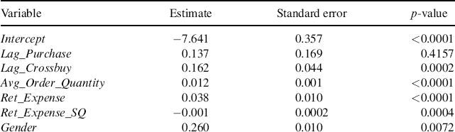

As we can see from the results, 8 of the 10 independent variables are significant at a p-value of 5% or better with only Lag_Purchase and Married being statistically non-significant. First, this means that Lag_Crossbuy positively affects current cross-buy, that is, customers who purchased across more categories in the previous quarter are more likely to cross-buy in the current quarter. Second, since the coefficient on Avg_Order_Quantity is positive and statistically significant, this means that customers who in the past have spent more on average are also more likely to cross-buy in the current time period. Third, we find a positive, but a diminishing, return on the effect of retention spending (Ret_Expense) on cross-buying in the same quarter since the coefficient on Ret_Expense is positive and the coefficient on Ret_Expense_SQ is negative. Fourth, we find that males are more likely to cross-buy than females. Fifth, we find a positive income effect suggesting that customers who have a higher income are more likely to cross-buy in the current quarter. Sixth, we find that customers who had a higher First_Purchase are more likely to cross-buy. Finally, since the coefficient on Loyalty is positive, this suggests that customers who are members of the loyalty program are more likely to cross-buy in the current quarter.
It is also important to understand exactly how changes in the drivers of cross-buy likelihood are likely to lead to either increases or decreases in cross-buy likelihood. To do this we need to determine the odds ratio for each of the parameter estimates. Since we are dealing with logistic regression, this means that we are interested in the log-odds ratio. For example, for Lag_Crossbuy, we want to know the change in cross-buy likelihood when Lag_Crossbuy = x and when Lag_Crossbuy = x + 1. For Lag_Crossbuy = x, we get the following:
![]()
and, for Lag_Purchase = 1,
![]()
By dividing the second equation by the first we get
![]()
We then simplify the equation to get the following:
![]()
When we compute the log-odds ratio for each of the statistically significant variables we get the following results for an increase in 1 unit of the independent variable. For the case of categorical variables such as Gender, the log-odds ratio is merely exp(βvariable).
| Variable | Log-odds ratio |
| Lag_Purchase | 1.176 |
| Avg_Order_Quantity | 1.012 |
| Ret_Expense | (0.037− 0.002*Ret_Expense) |
| Gender | 1.297 |
| Income | 1.262 |
| First_Purchase | 1.024 |
| Loyalty | 1.294 |
We gain the following insights from the log-odds ratios. With regard to Lag_Crossbuy, we see that each additional category a customer purchased in the previous quarter makes the customer 17.6% more likely to cross-buy in the current quarter. With regard to Avg_Order_Quantity, we see that for every increase in $1, the probability of cross-buying in the current quarter increases by 1.2%. With regard to Ret_Expense, we see that the odds ratio is dependent on the level of Ret_Expense. This is due to the fact that we include both the level and squared terms for Ret_Expense. For example, if we usually spend $15 on a given customer, by spending $16 we should see an increase in the likelihood of cross-buy by exp(0.037−0.002*16) = exp(0.005) = 1.005. This means that by increasing our spending from $15 to $16, we should see an increase in cross-buy likelihood by 0.5%. And, it is important to note that this will vary depending on the initial level of Ret_Expense. With regard to Gender, we see that males are 29.7% more likely to cross-buy than females. With regard to Income, we see that for each increase in Income level by 1 the cross-buy likelihood should increase by 26.2%. With regard to First_Purchase, we see that for each increase in $1, the likelihood of cross-buy increases by 2.4%. Finally, with regard to Loyalty, we see that by being a member of the loyalty program the probability of cross-buy in a given quarter is 29.4% higher than a customer that is not in the loyalty program.
Now that we have determined the drivers of cross-buying behavior by customers we need to use the output of the model to determine our model's predictive accuracy. To do this we need to use the estimates we obtained from the cross-buy model to help us determine the predicted probability that each customer will cross-buy. We use the parameter estimates from the cross-buy model and values for the x variables for each customer in each time period to predict whether a customer is likely to purchase in that time period. For a logistic regression we must apply the proper probability function as follows:
![]()
Once we compute the probability of cross-buy, we need to create a cutoff value to determine at which point we are going to divide the customers into the two groups – predicted to cross-buy and predicted not to cross-buy. There is no rule that explicitly tells us what that cutoff number should be. Often by default we select 0.5 since it equidistant from 0 and 1. However, it is also reasonable to check multiple cutoff values and choose the one that provide the best predictive accuracy for the dataset. By using 0.5 as the cutoff for our example, any customer whose predicted probability of cross-buy is greater than or equal to 0.5 is classified as predicted to cross-buy and the rest are predicted not to cross-buy. To determine the predictive accuracy we compare the predicted to the actual cross-buy values in a 2 × 2 table. For our sample of 500 customers over 11 quarters and 2678 purchase occasions (we drop quarter 1 since all customers purchased in quarter 1) we get Table 4.3.
Table 4.3 Predicted versus actual cross-buy.
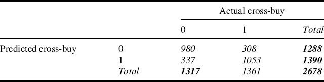
As we can see from the table, our in-sample model accurately predicts 74.4% of the customers who chose not to cross-buy on a given purchase occasion (980/1317) and 77.4% of the customers who chose to cross-buy on a given purchase occasion (1053/1361). This is a significant increase in the predictive capability of a random guess model2 which would be only 50.8% accurate for this dataset. Since our model is significantly better than the best alternative, in this case a random guess model, we determine that the predictive accuracy of the model is good. If there are other benchmark models available for comparison, the ‘best’ model would be the one which provides the highest accuracy of both the prediction to cross-buy and not to cross-buy, or in other words the prediction would provide the highest sum of the diagonal. In this case the sum of the diagonal is 2033 and it is accurate 75.9% of the time (2033/2678).
As a result we now know how changes in retention expense, past customer transactions, and customer characteristics are likely to either increase or decrease our likelihood of cross-buy. And we also know that these drivers do a good job in helping us predict whether a customer is going to cross-buy or not. This information can provide significant insights to managers who are charged with determining which customers are most likely to cross-buy.
4.5.2 How Do You Implement it?
To implement the logistic regression in this example we used the PROC Logistic feature in SAS. To determine predictive accuracy we carried out a SAS Data step and the Freq procedure. While we did use SAS to estimate the model and determine predictive accuracy, many other statistical packages are capable of estimating a logistic regression including (but not limited to) SPSS, MATLAB, and GAUSS.