
Chapter 2
The Implied Volatility Surface
Despite its flaws and limitations, the Black-Scholes model became the benchmark to interpret option prices. Specifically, option prices are reverse-engineered to calculate implied volatilities, the same way that bond prices are transformed into yields, which are easier to understand. This process, combined with interpolation and extrapolation techniques, gives rise to an entire surface along the strike and maturity dimensions.
2.1 The Implied Volatility Smile and Its Consequences
The Black-Scholes model assumes a single constant volatility parameter to price options. In practice, however, every listed vanilla option has a different implied volatility ![]() (K, T) for each strike K and maturity T. Figure 2.1 shows what an implied volatility surface
(K, T) for each strike K and maturity T. Figure 2.1 shows what an implied volatility surface ![]() looks like.
looks like.
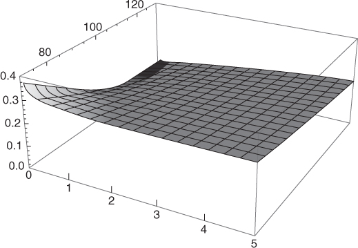
Figure 2.1 Implied volatility surface of the S&P 500 as of July 18, 2012. Strikes are in percentage of the spot level.
For a fixed maturity T the curve ![]() is called the implied volatility smile or skew and exhibits a downward-sloping shape, as shown in Figure 2.2. Note that in other asset classes, such as interest rates or currencies, the smile tends to be symmetric rather than downward-sloping.
is called the implied volatility smile or skew and exhibits a downward-sloping shape, as shown in Figure 2.2. Note that in other asset classes, such as interest rates or currencies, the smile tends to be symmetric rather than downward-sloping.

Figure 2.2 Implied volatility smile of S&P 500 index options expiring December 20, 2014, as of July 22, 2012.
Data source: Bloomberg.
2.1.1 Consequence for the Pricing of Call and Put Spreads
A direct consequence of the implied volatility smile is that the Black-Scholes model gives inaccurate call spread and put spread prices. To illustrate this point, Figure 2.3 shows the Black-Scholes price of a one-year call spread with strikes $100 and $110 as a function of the single Black-Scholes volatility parameter σ. We can see that the curve peaks at σ ≈ 30.8% for a maximum price of $3.78. Thus, no single value of σ may reproduce any market price above $3.78. Interestingly, this phenomenon is not symmetric: $90–$100 put spreads can be priced with a single volatility parameter, but the value of σ will be significantly off the level of implied volatility for each put.

Figure 2.3 Black-Scholes value of a call spread as a function of volatility. Spot price $100, one-year maturity, strikes $100 and $110, zero rates and dividends.
2.1.2 Consequence for Hedge Ratios
The smile does not mean that Black-Scholes is wrong and should be rejected. Practitioners typically price over-the-counter (OTC) vanilla options using Black-Scholes and an appropriate volatility interpolation or extrapolation scheme, for the simple reason that implied volatilities are derived from listed option prices in the first place. In other words, the fact that the Black-Scholes model may be faulty is fairly irrelevant for vanilla option pricing.
However, the vanilla hedge ratios or Greeks are model-dependent and should be adjusted for the smile. To see this, notice first how a change in spot price impacts the moneyness of an option: after a $1 uptick from an initial $100 underlying spot price, an out-of-the-money call struck at $110 is now only $9 out of the money. In the presence of the smile, we may want to use a different implied volatility to reprice the call, and we must make an assumption on the behavior of the smile curve:
- If we assume that the smile curve does not change at all, we should use the same implied volatility to reprice the call. This is known as the sticky-strike rule and produces the same delta as Black-Scholes.
- If we assume that the smile curve does not change with respect to moneyness (strike over spot), we should use the implied volatility of the 110/101 × 100 ≈ $108.91 call to reprice the call. This is known as the sticky-moneyness rule and produces a higher delta than Black-Scholes.
- If we assume that the smile curve does not change with respect to delta, we should use the implied volatility corresponding to the new delta to reprice the call. This is known as the sticky-delta rule and produces a higher delta than Black-Scholes. Note that the consistent definition of delta is circular in this case.
Other rules would obviously produce different results.
2.1.3 Consequence for the Pricing of Exotics
In Chapter 3 we will see that European exotic payoffs can in theory be replicated by a static portfolio of vanilla options along a continuum of strikes. In the absence of arbitrage, the price of the exotic option must match the price of the portfolio. Thus it would be inaccurate to use the Black-Scholes model to price the exotic option in the presence of the smile.
As a fundamental example consider the digital option that pays off $1 at maturity T if the final spot price ST is above the strike K, and 0 otherwise. The Black-Scholes value for the digital option is simply:

where S is the spot price, r is the continuous interest rate for maturity T, and σ is the constant Black-Scholes volatility parameter.
Digital options are difficult to delta-hedge because their delta becomes very large around the strike as maturity approaches. Equity exotic traders will typically overhedge them with tight call spreads. For example, to overhedge a digital paying off $1,000,000 above a strike of $100 and 0 otherwise, a trader might buy 200,000 call spreads with strikes $95 and $100.
Figure 2.4 shows how in general a quantity 1/ϵ of call spreads with strikes K − ϵ and K will overhedge a digital option struck at K. In the limit as ϵ goes to zero, we obtain an exact hedging portfolio whose price is:
where σ*(K, T) is the implied volatility for strike K and maturity T and VBS is the Black-Scholes vega of a vanilla option. Because the equity smile is mostly downward-sloping we typically have ![]() and thus the digital option is worth more than its Black-Scholes value.
and thus the digital option is worth more than its Black-Scholes value.

Figure 2.4 Digital and leveraged call spread payoffs.
2.2 Interpolation and Extrapolation
Implied volatilities derived from listed option prices are only available for a finite number of listed strikes and maturities. However, on the OTC market, option investors will ask for quotes for any strike or maturity, and it is important to be able to interpolate or extrapolate implied volatilities.
Interpolation is relatively easy: for a given maturity, if the at-the-money option has 20% implied volatility and the $90-strike option has 25% implied volatility, it intuitively makes sense to linearly interpolate and say that the $95-strike option should have a 22.5% implied volatility. Similarly, for a given strike, we can linearly interpolate implied volatility through time.
One issue with linear interpolation, however, is that it produces a cracked smile curve. More sophisticated interpolation techniques, such as cubic splines, are often used to obtain a smooth curve. Figure 2.5 compares the two methods.
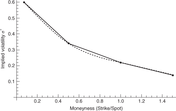
Figure 2.5 Comparison of linear (solid line) and cubic splines (dashed line) interpolation methods.
It must be emphasized that unconstrained interpolation methods may produce arbitrageable volatility surfaces. Several papers listed in Homescu (2011) discuss how to eliminate arbitrage.
On the other hand extrapolation is a difficult endeavor: how to price a five-year option if the longest listed maturity is two years? There is no definite answer to this question, and we must typically resort to a volatility surface model (see Section 2.4).
Note that extrapolating a cubic spline fit tends to produce unpredictable results and should be avoided at all costs.
2.3 Implied Volatility Surface Properties
Not every surface f(K, T) is a candidate for an implied volatility surface ![]() . Denote
. Denote ![]() the call and put values induced by
the call and put values induced by ![]() , respectively. To preclude arbitrage we must at least require:
, respectively. To preclude arbitrage we must at least require:
These1 inequalities place upper and lower bounds on ![]() and its derivatives. For example, by the chain rule applied to
and its derivatives. For example, by the chain rule applied to ![]() , we obtain
, we obtain ![]() , and thus
, and thus ![]() is equivalent to the upper bound
is equivalent to the upper bound ![]() .
.
When designing an implied volatility surface model, it is important to check that these constraints are satisfied.
The implied volatility surface must also satisfy certain asymptotic properties. Perhaps the most notable one for fixed maturity is that implied variance, the square of implied volatility, is bounded from above by a function linear in log-strike as kF → 0 and kF → ∞:
where kF = K/F is the forward-moneyness and β ∈ [0, 2] is different for each limit. This result is more rigorously expressed with supremum limits and we refer the interested reader to Lee (2004).
2.4 Implied Volatility Surface Models
Every large equity option house maintains several proprietary models of the implied volatility surface, which are used by their market-makers to mark positions. By definition these models are not in the public domain, and we must regrettably leave them in the dark. Fortunately some researchers have published their models and we now present a selection.
There are two ways to model the volatility surface ![]() :
:
- Directly, by specifying a functional form such as a parametric function, or an interpolation and extrapolation method;
- Indirectly, by modeling the behavior of the underlying asset differently from the geometric Brownian motion posited by Black-Scholes.
Here, it is worth distinguishing between two kinds of implied volatility ![]() : market-implied volatility
: market-implied volatility ![]() , which is computed from market prices; and model-implied volatility
, which is computed from market prices; and model-implied volatility ![]() , which is induced by a volatility surface model attempting to reproduce
, which is induced by a volatility surface model attempting to reproduce ![]() . However, for ease of notation we will often keep the notation σ* when there is no ambiguity nor need for such distinction.
. However, for ease of notation we will often keep the notation σ* when there is no ambiguity nor need for such distinction.
2.4.1 A Parametric Model of Implied Volatility: The SVI Model
A popular parameterization of the smile for fixed maturity is the SVI model by Gatheral (2004). SVI stands for stochastic volatility-inspired and has the simple functional form:

where a, b, ρ, m, and s are parameters depending on T, and kF = K/F is the forward-moneyness. Intuitively a controls the overall level of variance, m corresponds to a moneyness shift, ρ is related to the correlation between stock prices and volatility and controls symmetry, s controls the smoothness near the money (kF = 1), and b controls the angle between small and large strikes.
Figure 2.6 shows an example of the shape of the smile produced by the SVI model, which is plausible.

Figure 2.6 SVI fit of one-year implied volatility smile for the S&P 500 as of July 18, 2012. Black dots correspond to observed data.
The SVI model is connected to stochastic volatility models (see Gatheral-Jacquier (2011)). Specifically, the authors show how Equation (2.4) is the limit-case of the implied volatility smile produced by the Heston model as the maturity goes to infinity.
To ensure the no-arbitrage condition Equation (2.1) we must have ![]() . In his original 2004 talk, Gatheral claims that this condition is also sufficient to ensure Equation (2.2), but a recent report by Roper (2010) suggests otherwise.
. In his original 2004 talk, Gatheral claims that this condition is also sufficient to ensure Equation (2.2), but a recent report by Roper (2010) suggests otherwise.
An attractive property of the SVI model is that it is relatively easy to satisfy Equation (2.3) since its parameters are time dependent. This is also a drawback: as a surface, the SVI model has too many parameters. To circumvent this issue, Gurrieri (2011) put forward a class of arbitrage-free SVI models with term structure using 11 time-homogenous parameters.
It should be noted that, being a function of ![]() and thus
and thus ![]() , the SVI model incorporates the sticky-delta rule and thus produces a higher delta than Black-Scholes, as shown in Figure 2.7.
, the SVI model incorporates the sticky-delta rule and thus produces a higher delta than Black-Scholes, as shown in Figure 2.7.
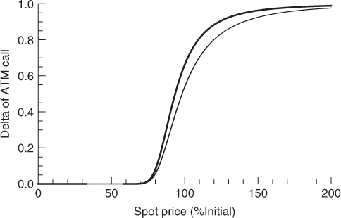
Figure 2.7 The SVI model of the implied volatility surface produces a higher delta than Black-Scholes.
2.4.2 Indirect Models of Implied Volatility
Any alternative to Black-Scholes will generate an implied volatility surface, which may be used to appraise the quality of the model. This is a major source of implied volatility surface models.
2.4.2.1 The SABR Model
The stochastic alpha, beta, rho (SABR) model of Hagan and colleagues (2002) assumes that the underlying forward price dynamics are described by the coupled diffusion equations:

where W and Z are standard Brownian motions with ![]() and α, β, ρ are constant model parameters.
and α, β, ρ are constant model parameters.
In the special case β = 1 an analytical formula for implied volatility is available for short maturities, which allows to fit the parameters to observed option prices. Near the money the formula has the Taylor expansion expression:
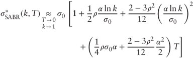
The SABR model is popular for interest rates where the smile is more symmetric than for equities.
2.4.2.2 The Heston Model
The Heston (1993) model is perhaps the most popular approach for stochastic volatility. It assumes the following underlying spot price dynamics coupled to an instantaneous variance process:
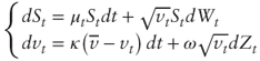
where W and Z are standard Brownian motions with ![]() and
and ![]() are constant model parameters that must satisfy the Feller condition
are constant model parameters that must satisfy the Feller condition ![]() to ensure strictly positive instantaneous variance vt at all times. The instantaneous rate of return μt on the underlying asset can be anything since it will disappear under the risk-neutral measure.
to ensure strictly positive instantaneous variance vt at all times. The instantaneous rate of return μt on the underlying asset can be anything since it will disappear under the risk-neutral measure.
Rouah (2013) provides a valuable resource detailing the theoretical and practical aspects of the Heston model, including code examples.
Although no analytical formula for implied volatility is available, the popularity of the Heston model is largely due to the existence of quasi-analytical formulas for European options making the computation of implied volatilities very quick.
Figure 2.8 compares a Heston fit to the S&P 500 implied volatility surface. We can see that the Heston model produces a plausible shape but is too flat for short expiries.
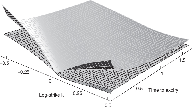
Figure 2.8 Comparison of the S&P 500 implied volatility surface (top) with its Heston fit (bottom) as of September 15, 2005.
Source: Jim Gatheral, The Implied Volatility Surface: A Practitioner's Guide (Hoboken, NJ: John Wiley & Sons, 2005). Reprinted with permission of John Wiley & Sons, Inc.
One limitation of the Heston model is that instantaneous variance is a somewhat elusive concept, which cannot be measured in practice. However an analytical formula for the total expected variance over a period [0, T] is available:

Hence the expected total annualized variance is approximately constant at v0 regardless of maturity, which is inconsistent with empirical market observations (see Section 5.2).
2.4.2.3 The LNV Model
Recently Carr and Wu (2011) proposed a sophisticated framework for the underlying forward price dynamics, which results in a closed-form formula for implied volatility. The forward price process solves the diffusion equation:
where W is a standard Brownian motion and v is an arbitrary stochastic instantaneous variance process. Furthermore, the entire implied volatility surface ![]() is assumed to evolve through time according to the diffusion equation:
is assumed to evolve through time according to the diffusion equation:
where Z is a standard Brownian motion with ![]() and μ, ω, ρ may be stochastic.
and μ, ω, ρ may be stochastic.
Carr-Wu then show that in this setup the implied volatility surface at any time t is fully determined by a quadratic equation, which depends on μt, ωt, ρt and the unspecified vt.
This very general framework can produce a wide range of implied volatility surfaces. Choosing ![]() and
and ![]() yields the Log-Normal Variance (LNV) model in which
yields the Log-Normal Variance (LNV) model in which ![]() is solution to the quadratic equation:
is solution to the quadratic equation:

where κ, w, η, θ, v, ρ are constant parameters and k denotes moneyness K/S0.
The LNV model thus combines two attractive features: a functional parametric form for the implied volatility, and known dynamics for the evolution of the underlying spot price as well as the implied volatility surface itself.
References and Bibliography
- Carr, Peter, and Liuren Wu. 2011. “A New Simple Approach for Constructing Implied Volatility Surfaces.” Working paper, New York University and Baruch College.
- Derman, Emanuel. 2010. “Introduction to the Volatility Smile.” Lecture notes, Columbia University.
- Gatheral, Jim. 2004. “A Parsimonious Arbitrage-Free Implied Volatility Parameterization with Application to the Valuation of Volatility Derivatives.” Proceedings of the Global Derivatives and Risk Management 2004 Madrid conference.
- Gatheral, Jim. 2005. The Implied Volatility Surface: A Practitioner's Guide. Hoboken, NJ: John Wiley & Sons.
- Gatheral, Jim, and Antoine Jacquier. 2011. “Convergence of Heston to SVI.” Quantitative Finance 11 (8): 1129–1132.
- Gurrieri, Sébastien. 2011. “A Class of Term Structures for SVI Implied Volatility.” Working paper. Available at http://ssrn.com/abstract=1779463 or http://dx.doi.org/10.2139/ssrn.1779463.
- Hagan, Patrick S., Deep Kumar, Andrew L. Lesniewski, and Diana E. Woodward. 2002. “Managing Smile Risk.” Wilmott Magazine (September): 84–108.
- Heston, Stephen L. 1993. “A Closed-Form Solution for Options with Stochastic Volatility with Applications to Bond and Currency Options.” Review of Financial Studies 6 (2): 327–343.
- Hodges, Hardy M. 1996. “Arbitrage Bounds on the Implied Volatility Strike and Term Structures of European-Style Options.” Journal of Derivatives (Summer): 23–35.
- Homescu, Cristian. 2011. “Implied Volatility Surface: Construction Methodologies and Characteristics.” Available at http://arxiv.org/abs/1107.1834v1.
- Karlin, Samuel, and Howard M. Taylor. 1981. “Diffusion Processes.” In A Second Course in Stochastic Processes, 157–396. San Diego, CA: Academic Press.
- Lee, Roger. 2004. “The Moment Formula for Implied Volatility at Extreme Strikes.” Mathematical Finance 14: 469–480.
- Roper, Michael. 2010. “Arbitrage Free Implied Volatility Surfaces.” Working paper. Available at www.maths.usyd.edu.au/u/pubs/publist/preprints/2010/roper-9.pdf.
- Rouah, Fabrice. 2013. The Heston Model in Matlab and C#. Hoboken, NJ: John Wiley & Sons.
- Zeliade Systems. 2009. “Quasi-Explicit Calibration of Gatheral's SVI model.” Zeliade White Paper.
Problems
2.1 No Call or Put Spread Arbitrage Condition
Consider an underlying asset S with spot price S and forward price F. Let r denote the continuous interest rate for maturity T, ![]() be the upper and lower bounds on the slope of the smile corresponding to the no call or put spread arbitrage condition (2.1). Given
be the upper and lower bounds on the slope of the smile corresponding to the no call or put spread arbitrage condition (2.1). Given ![]() , show that that
, show that that ![]() where
where ![]() .
.
2.2 No Butterfly Spread Arbitrage Condition
Assume zero interest rates and dividends. Consider the Black-Scholes formula for the European call struck at K with maturity T:

where S is the underlying asset's spot price, σ is the volatility parameter, and N(.) is the cumulative distribution function of a standard normal.
- Given
 , derive the identities:
- A second-order chain rule. Show that if f(x, y) and u(t) are C2 (twice continuously differentiable) then the second-order derivative of ϕ(t) = f(t, u(t)) is given as:
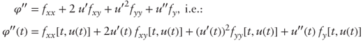
- where fxx, fxy, and fyy denote the second-order partial derivatives of f.
- Assume that the implied volatility smile σ*(K) is C2 for a given maturity T. Using your results in (a) and (b), show that for
 :
:
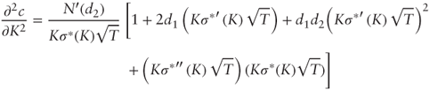
- What does the no butterfly arbitrage condition (2.2) reduce to?

2.3 Sticky True Delta Rule
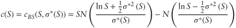
Consider a one-year vanilla call with strike K = 1, and let ![]() (S) be its implied volatility at various spot price assumptions S. Assume zero rates and dividends and denote the call price:
(S) be its implied volatility at various spot price assumptions S. Assume zero rates and dividends and denote the call price:
- a. Show that the option's delta Δ is
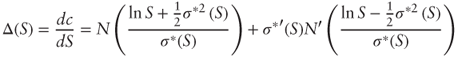
- Assume that
 is a linear function of Δ:
  . Show that Δ is solution to the first-order differential equation:

- Is Δ higher or lower than the Black-Scholes delta?
2.4 SVI Fit
Using your favorite optimization software (Matlab, Mathematica, etc.) find the parameters for the SVI model corresponding to a least square fit of the following one-year implied volatility data:
| Strike (%forward) | 20% | 50% | 70% | 90% | 100% | 110% | 130% | 150% | 160% |
| Implied volatility | 45.5% | 34.6% | 29.4% | 24.0% | 22.3% | 19.9% | 16.4% | 14.9% | 14.3% |
Answer: a = 0.0180, b = 0.0516, ρ = −0.9443, m = 0.2960, s = 0.1350 using initial condition a = 0.04, b = 0.4, ρ = −0.4, m = 0.05, s = 0.1, and bounds a > 0, 0 < b < 2, −1 < ρ < 1, s > 0.