
Chapter 3
Implied Distributions
Perhaps the favorite activity of quantitative analysts is to decode market data into information about the future upon which a trader can base his or her decisions. This is the purpose of the implied distribution that translates option prices into probabilities for the underlying stock or stock index to reach certain levels in the future. In this chapter, we derive the implied distribution and show how it may be exploited to price and hedge certain exotic payoffs.
3.1 Butterfly Spreads and the Implied Distribution
Vanilla option prices contain probability information about the market's guess at the future level of the underlying asset S. For example, suppose that Kroger Co. trades at $24 and that one-year calls struck at $24 and $25 trade at $1 and $0.60 respectively. If interest rates are zero, we may then infer that the probability of the terminal spot price ST in one year to be above $24 must satisfy:
because the digital payoff ![]() dominates the call spread as shown in Figure 3.1.
dominates the call spread as shown in Figure 3.1.
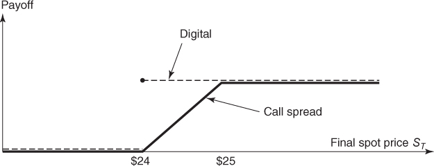
Figure 3.1 The digital payoff dominates the call spread payoff.
Similarly the price of a butterfly spread with strikes $23, $24, and $25 (i.e., long one call struck at $23, short two calls struck at $24, and long one call struck at $25) will give a lower bound for ![]() as shown in Figure 3.2.
as shown in Figure 3.2.
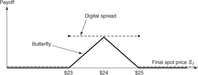
Figure 3.2 The digital spread payoff dominates the butterfly spread payoff.
Generally, if all option prices are available along a continuum of strikes—such as option prices generated by an implied volatility surface model—we may consider butterfly spreads with strikes ![]() leveraged by 1/ϵ2 and obtain in the limit as ϵ → 0 the implied distribution density of ST:
leveraged by 1/ϵ2 and obtain in the limit as ϵ → 0 the implied distribution density of ST:
where r is the continuous interest rate for maturity T, and c(K) denotes the price of the call struck at K.
Note that by put-call parity we have ![]() and thus put prices may alternatively be used to compute the implied distribution density.
and thus put prices may alternatively be used to compute the implied distribution density.
Figure 3.3 compares the Black-Scholes lognormal density to the implied distribution density generated by an SVI model fit of S&P 500 option prices with about 2.4-year maturity. We can see that the implied density is skewed toward the right and has a fatter left tail.
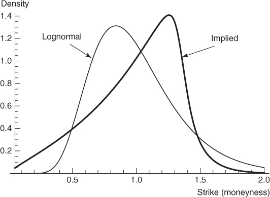
Figure 3.3 The lognormal and implied distribution densities.
The implied distribution density may be obtained directly from a smooth volatility surface ![]() by differentiating
by differentiating ![]() twice with respect to K (see Problem 2.4.2 (c)). The corresponding formula is:
twice with respect to K (see Problem 2.4.2 (c)). The corresponding formula is:
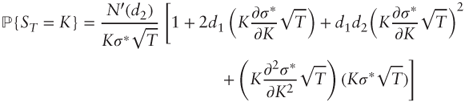
where ![]() , F is the forward price of S for maturity T, and N′(·) is the standard normal distribution density. It is worth emphasizing that Equation (3.2) relies on partial derivatives of σ* with respect to the dollar strike K, and that one must be careful when using an implied volatility model such as the SVI model, which is based on forward-moneyness kF = K/F. In the latter case, we must substitute
, F is the forward price of S for maturity T, and N′(·) is the standard normal distribution density. It is worth emphasizing that Equation (3.2) relies on partial derivatives of σ* with respect to the dollar strike K, and that one must be careful when using an implied volatility model such as the SVI model, which is based on forward-moneyness kF = K/F. In the latter case, we must substitute ![]() and
and ![]() .
.
The first factor, ![]() , is the Black-Scholes lognormal distribution at point K using implied volatility. Without the second factor between brackets, the integral does not sum to 1, unless the smile is flat.
, is the Black-Scholes lognormal distribution at point K using implied volatility. Without the second factor between brackets, the integral does not sum to 1, unless the smile is flat.
The implied distribution reveals what options markets “think” in terms of the future evolution of the underlying asset price. It is a useful theoretical concept, but in practice it can be difficult to exploit this information for trading.
3.2 European Payoff Pricing and Replication
Consider an option with arbitrary European payoff f(ST) at maturity T, and let ![]() be the implied distribution density. The corresponding option value is then
be the implied distribution density. The corresponding option value is then ![]() and by direct substitution of Equation (3.1) we obtain the Breeden-Litzenberger (1978) formula:
and by direct substitution of Equation (3.1) we obtain the Breeden-Litzenberger (1978) formula:
The knowledge of the implied distribution thus allows us to value any European option consistently with the vanilla option market. It turns out that this value is in fact an arbitrage price, at least in theory when we can trade all vanilla options along a continuum of strikes K > 0.
To see this, assume that f is bounded and smooth (twice continuously differentiable) to perform an integration by parts and write:
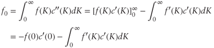
because infinite-strike calls are worthless. Integrating by parts again yields:
Furthermore zero-strike calls are always worth ![]() ; additionally, by put-call parity
; additionally, by put-call parity ![]() , thus by differentiation
, thus by differentiation ![]() and since zero-strike puts are worthless we have
and since zero-strike puts are worthless we have ![]() . Substituting into the previous equation we get:
. Substituting into the previous equation we get:
This expression suggests that the option may be hedged with a portfolio:
- Long zero-coupon bonds in quantity f(0)e–rT
- Long zero-strike calls in quantity f′(0)
- Long all vanilla calls struck at K > 0 in quantities

The definite proof of this result is provided by establishing that the option payoff perfectly matches the portfolio payoff:
which simply turns out to be the first-order Taylor expansion of f over [0, ST] with remainder in integral form after noticing that the bounds of the integral are actually 0 and ST.
An alternative approach mixing puts and calls is developed in Problem 3.4.2.
This is a strong fundamental result that directs how to price and hedge European payoffs, with the following limitations:
- It only applies to European payoffs. Other option payoffs that depend on the history of the underlying asset price (such as Asian or barrier options) or have an early exercise feature (such as American options) require more sophisticated valuation methods and cannot be perfectly replicated with a static portfolio of vanilla options.
- In practice, only a finite number of strikes are available. While it is possible to overhedge convex payoffs with a finite portfolio of vanillas, exact replication cannot be achieved.
3.3 Pricing Methods for European Payoffs
As stated earlier, the implied distribution ![]() makes it possible to price any European payoff f(ST). Several numerical integration methods, such as the trapezoidal method, are then available to compute
makes it possible to price any European payoff f(ST). Several numerical integration methods, such as the trapezoidal method, are then available to compute ![]() . One issue is that these methods become inefficient in large dimensions (i.e., multi-asset payoffs), which is the topic of Chapters 6 to 9.
. One issue is that these methods become inefficient in large dimensions (i.e., multi-asset payoffs), which is the topic of Chapters 6 to 9.
Another approach is Monte Carlo simulation, which is easy to generalize to multiple dimensions. Using a cutoff A ![]() 0 we may approximate f0 by:
0 we may approximate f0 by:

where u1,…, un are n independent simulations from a uniform distribution over [0, 1].
We can improve this approach by means of the importance sampling technique, which exploits the fact that the implied distribution is bell-shaped and somewhat similar to the Black-Scholes lognormal distribution ![]() with sensible volatility parameter σ (e.g., at-the-money implied volatility for maturity T). To do so, rewrite:
with sensible volatility parameter σ (e.g., at-the-money implied volatility for maturity T). To do so, rewrite:
where X is lognormally distributed with density ![]() (K) and x1,…, xn are simulated values of X. The ratio
(K) and x1,…, xn are simulated values of X. The ratio ![]() measures how close the implied and lognormal distributions are.
measures how close the implied and lognormal distributions are.
Simulating X is straightforward through the identity ![]() where
where ![]() is a standard normal, for which there are many efficient pseudo-random generators. For completeness we provide the Matlab code to price the “capped quadratic” payoff according to the implied distribution shown in Figure 3.3.
is a standard normal, for which there are many efficient pseudo-random generators. For completeness we provide the Matlab code to price the “capped quadratic” payoff according to the implied distribution shown in Figure 3.3.
function price = ImpDistMC(n)
  %Note: this algorithm assumes zero rates and dividends
  epsilon = 0.0001;
  T = 2.41; %maturity
  function val = Payoff(S)
    val = min(1, S∧2);
   end
  function vol = SVI(k)
    a = 0.02;
    b = 0.05;
    rho = -1;
    m = 0.3;
    s = 0.1;
    k = log(k);
    vol = sqrt( a + b*( rho*(k-m) + sqrt( (k-m)∧2 + s∧2 ) ) );
  end
  function density = ImpDist(k)
    vol = SVI(k);
    volPrime = (SVI(k+epsilon)-vol)/epsilon;                  %finite difference
    volDblPrime = (SVI(k+epsilon)-2*vol+SVI(k-epsilon))/epsilon∧2;                  %finite diff.
    d1 = (-log(k)+0.5*vol∧2*T)/(vol*sqrt(T));
    d2 = d1 - vol*sqrt(T);
    density = normpdf(d2)/(k*vol*sqrt(T)) * (1 + …             2*d1*k*volPrime*sqrt(T) + …
               d1*d2*(k*volPrime*sqrt(T))∧2 + …             (k*volDblPrime*sqrt(T))*(k*vol*sqrt(T)) );
  end
    %%%%%%%%%%%%%%%%%%%%%%%%%%
    %%% MAIN FUNCTION BODY %%%
    %%%%%%%%%%%%%%%%%%%%%%%%%%
  atm_vol = SVI(1);
  price = 0;
  for i=1:n
    x = exp(atm_vol*randn*sqrt(T) - 0.5*atm_vol∧2*T);
                %lognormal simulation
    price = (i-1)/i*price + Payoff(x)*ImpDist(x) …
          / lognpdf(x,-0.5*atm_vol∧2*T,atm_vol*sqrt(T)) / i;
  end
end
3.4 Greeks
Because the implied distribution is derived from vanilla option prices in the first place, it produces the same delta as the input volatility smile. Consequently, if the implied volatility smile incorporates a sticky-delta rule, the delta obtained by repricing calls using the implied distribution will be higher than the Black-Scholes delta.
The implied distribution also makes it possible to calculate smile-consistent Greeks for any European payoff. In practice this is often done using finite differences, but one must be careful with the numerical precision of the method used for pricing. In particular the Monte Carlo method has error of order ![]() where n is the number of simulations, and will generate a different price on each call unless the pseudo-random generator is systematically initialized at the same seed.
where n is the number of simulations, and will generate a different price on each call unless the pseudo-random generator is systematically initialized at the same seed.
It is worth emphasizing that the implied distribution depends on the variables or parameters used for the Greeks. For example, if the payoff f(ST) is independent from the initial spot price S0 the delta may be written ![]() which involves the derivative of the implied distribution with respect to the spot price.
which involves the derivative of the implied distribution with respect to the spot price.
References
- Breeden, Douglas T., and Robert H. Litzenberger. 1978. “Prices of State-Contingent Claims Implicit in Option Prices.” Journal of Business 51 (4): 621–651.
- Demeterfi, Kresimir, Emanuel Derman, Michael Kamal, and Joseph Zhou. 1999. “More than You Ever Wanted to Know about Volatility Swaps.” Goldman Sachs Quantitative Strategies Research Notes, March.
Problems
3.1 Overhedging Concave Payoffs
Consider a concave payoff f(ST) over an interval [S–, S+]. Propose a method to overhedge this payoff using a finite portfolio of vanilla calls.
3.2 Perfect Hedging with Puts and Calls
Show that for any smooth (twice continuously differentiable) payoff f(ST):
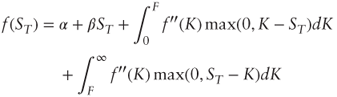
where F is the forward price and α and β are constants to be identified. What is the corresponding option price f0?
3.3 Implied Distribution and Exotic Pricing
- Reproduce Figure 3.3 using T = 2.4 and the following parameters for the SVI model: a = 0.02, b = 0.05, ρ = –1, m = 0.3, s = 0.1. Assume S0 = 1 as well as zero interest and dividend rates.
- Using a numerical integration algorithm check the price of the “capped quadratic” option, then compute the price of the following option payoffs:

 , where C = 25%. Then solve for C to obtain a price of 100%.
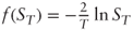 . What is
  ?
?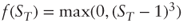 . Then find a vanilla overhedge over the interval [0,2] with strikes 0.5, 0.9, 1, 1.1, 1.3, 1.7 and compare the price of the overhedge with the theoretical price.
3.4 Conditional Pricing
On August 24, 2012, Kroger Co.'s stock traded at $21.795, and options maturing in 511 days had the following implied volatilities:
| Strike (%Spot) | 30% | 50% | 70% | 90% | 100% | 110% | 130% | 150% | 200% |
| Impl. Vol. (%) | 49.58 | 36.59 | 30.17 | 25.43 | 24.23 | 22.97 | 21.40 | 20.86 | 22.89 |
The forward price was $21.366, and the continuous interest rate was 0.81%.
- Calibrate the SVI model parameters to this data. Answer: a = 0, b = 0.1272, ρ = – 0.7249, m = –0.1569, s = 0.5388 using initial condition a = 0.04, b = 0.4, ρ = –0.4, m = 0.05, s = 0.1, and bounds a > 0, 0 < b < 2.024, –1 < ρ < 1, s > 0.
- Produce the graph of the corresponding implied distribution and compute the price of the “capped quadratic” option with payoff
 using the numerical method of your choice. Answer: approximately $0.797.
 - The following graph (Figure 3.6) shows the history of Kroger Co.'s stock price since 1980. Based on this graph, you reckon that the stock price will remain above $14 within the next three years.
- Compute the probability that ST > 14 using the implied distribution.
- Compute the value of the “capped quadratic” option conditional upon {ST > 14}. Is this an arbitrage price?
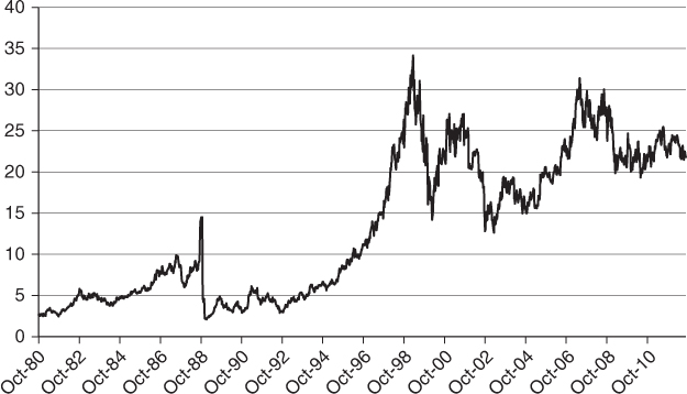
Figure 3.6 Historical price of Kroger Co.'s stock since 1980.
3.5 Path-Dependent Payoff
Consider an option whose payoff at maturity T2 is a nonlinear function ![]() of the future underlying spot price observed at times T1 < T2.
of the future underlying spot price observed at times T1 < T2.
- Give two classical examples of such an option.
- Write the pseudo-code to price this option in the Black-Scholes model using the Monte Carlo method.
- Assume that the implied distributions of both
 and
and  are known. Can you think of a method to find “the” value of the option? If yes provide the pseudo-code; if not explain what information you are missing.
3.6 Delta
Modify the code from Section 3-3 to calculate the delta of the “capped quadratic” option. Hint: Write ![]() and carefully amend Equation (3.2) accordingly.
and carefully amend Equation (3.2) accordingly.