2 RANDOM VARIABLES AND THEIR PROBABILITY DISTRIBUTIONS
2.1 INTRODUCTION
In Chapter 1 we dealt essentially with random experiments which can be described by finite sample spaces. We studied the assignment and computation of probabilities of events. In practice, one observes a function defined on the space of outcomes. Thus, if a coin is tossed n times, one is not interested in knowing which of the 2n n-tuples in the sample space has occurred. Rather, one would like to know the number of heads in n tosses. In games of chance one is interested in the net gain or loss of a certain player. Actually, in Chapter 1 we were concerned with such functions without defining the term random variable. Here we study the notion of a random variable and examine some of its properties.
In Section 2.2 we define a random variable, while in Section 2.3 we study the notion of probability distribution of a random variable. Section 2.4 deals with some special types of random variables, and Section 2.5 considers functions of a random variable and their induced distributions.
The fundamental difference between a random variable and a real-valued function of a real variable is the associated notion of a probability distribution. Nevertheless our knowledge of advanced calculus or real analysis is the basic tool in the study of random variables and their probability distributions.
2.2 RANDOM VARIABLES
In Chapter 1 we studied properties of a set function P defined on a sample space (Ω,
). Since P is a set function, it is not very easy to handle; we cannot perform arithmetic or algebraic operations on sets. Moreover, in practice one frequently observes some function of elementary events. When a coin is tossed repeatedly, which replication resulted in heads is not of much interest. Rather one is interested in the number of heads, and consequently the number of tails, that appear in, say, n tossings of the coin. It is therefore desirable to introduce a point function on the sample space. We can then use our knowledge of calculus or real analysis to study properties of P.
In order to verify whether a real-valued function on (Ω,
) is an RV, it is not necessary to check that (1) holds for all Borel sets B ∈
. It suffices to verify (1) for any class
of subsets of
which generates
. By taking
to be the class of semiclosed intervals
we get the following result.
PROBLEMS 2.2
Let X be the number of heads in three tosses of a coin. What is Ω? What are the values that X assigns to points of Ω? What are the events
?
A die is tossed two times. Let X be the sum of face values on the two tosses and Y be the absolute value of the difference in face values. What is Ω? What values do X and Y assign to points of Ω? Check to see whether X and Y are random variables.
Let X be an RV. Is |X| also an RV? If X is an RV that takes only nonnegative values, is
also an RV?
A die is rolled five times. Let X be the sum of face values. Write the events
.
Let
and
be the Borel σ–field of subsets of Ω. Define X on Ω as follows:
if
, and
if
. Is X an RV? If so, what is the event
?
Let
be a class of subsets of
which generates
. Show that X is an RV on Ω if and only if X-1(A) ∈
for all A ∈
.
2.3 PROBABILITY DISTRIBUTION OF A RANDOM VARIABLE
In Section 2.2 we introduced the concept of an RV and noted that the concept of probability on the sample space was not used in this definition. In practice, however, random variables are of interest only when they are defined on a probability space. Let (Ω,
,P) be a probability space, and let X be an RV defined on it.
and it follows that the number of points x in (a, b] with jump
is atmost ε– 1{F(b)–F(a)}. Thus, for every integer N, the number of discontinuity points with jump greater than 1/N is finite. It follows that there are no more than a countable number of discontinuity points in every finite interval (a, b]. Since
is a countable union of such intervals, the proof is complete.
Finally, let {xn} be a sequence of numbers decreasing to –∞. Then,
and
Therefore,
Similarly,
and the proof is complete.
The next result, stated without proof, establishes a correspondence between the induced probability Q on (
,
) and a point function F defined on
.
and
PROBLEMS 2.3
Write the DF of RV X defined in Problem 2.2.1, assuming that the coin is fair.
What is the DF of RV Y defined in Problem 2.2.2, assuming that the die is not loaded?
Do the following functions define DFs?
, and = 1 if
.
.
, and
.
if
, and
.
Let X be an RV with DF F.
If F is the DF defined in Problem 3(a), find
.
If F is the DF defined in Problem 3(d), find
.
2.4 DISCRETE AND CONTINUOUS RANDOM VARIABLES
Let X be an RV defined on some fixed, but otherwise arbitrary, probability space (Ω,
, P), and let F be the DF of X. In this book, we shall restrict ourselves mainly to two cases, namely, the case in which the RV assumes at most a countable number of values and hence its DF is a step function and that in which the DF F is (absolutely) continuous.
Then
.
We next consider RVs associated with DFs that have no jump points. The DF of such an RV is continuous. We shall restrict our attention to a special subclass of such RVs.
PROBLEMS 2.4
Let
Does {pk} define the PMF of some RV? What is the DF of this RV? If X is an RV with PMF {pk}, what is P{n ≤ X ≤ N}, where n, N (N > n) are positive integers?
In Problem 2.3.3, find the PDF associated with the DFs of parts (b), (c), and (d).
Does the function
if
, and
if
, where
, define a PDF? Find the DF associated with fθ (x); if X is an RV with PDF fθ(x), find
.
Does the function
if
, and
otherwise, where
define a PDF? Find the corresponding df.
For what values of K do the following functions define the PMF of some RV?
Show that the function
is a PDF. Find its DF.
For the PDF
if
, and
if
, find
.
Which of the following functions are density functions:
, and 0 elsewhere.
, and 0 elsewhere.
, and 0 elsewhere,
.
,
, and 0 elsewhere.
for
for
for
,
for
, = 4/27 for
, and 0 elsewhere.
.
(c), (d), and (f)
Are the following functions distribution functions? If so, find the corresponding density or probability functions.
for
,
for
,
for
,
for
and =1 for
.
if
,
if
, and 1 for
where
Suppose
is given for a random variable X (of the continuous type) for all x. How will you find the corresponding density function? In particular find the density function in each of the following cases:
if
, and
for
,
is a constant.
if
, and
, for
,
is a constant.
if
, and
if
.
if
, and
if
;
and
are constants.
2.5 FUNCTIONS OF A RANDOM VARIABLE
Let X be an RV with a known distribution, and let g be a function defined on the real line. We seek the distribution of
, provided that Y is also an RV. We first prove the following result.
Example 4 shows that we need some conditions on g to ensure that g(X) is also an RV of the continuous type whenever X is continuous. This is the case when g is a continuous monotonic function. A sufficient condition is given in the following theorem.
In Examples 7 and 8 the function
can be written as the sum of two monotone functions. We applied Theorem 3 to each of these monotonic summands. These two examples are special cases of the following result.
A similar computation can be made for
. It follows that the PDF of Y is given by
PROBLEMS 2.5
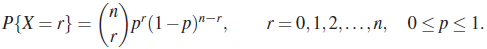
Let X be a random variable with probability mass function
Find the PMFs of the RVs (a)
, (b)
, and (c)
.
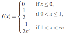
Let X be an RV with PDF
Find the PDF of the RV 1/X.
Let X be a positive RV of the continuous type with PDF f(·). Find the PDF of the RV
. If, in particular, X has the PDF
what is the PDF of U?
Let X be an RV with PDF f defined by Example 11. Let
and
. Find the DFs and PDFs of Y and Z.
Let X be an RV with PDF
where
. Let
. Find the PDF of Y.
A point is chosen at random on the circumference of a circle of radius r with center at the origin, that is, the polar angle θ of the point chosen has the PDF
Find the PDF of the abscissa of the point selected.
For the RV X of Example 7 find the PDF of the following RVs: (a)
, (b)
, and (c)
, where
if
, = 1/2 if
, and = –1 if
.
Suppose that a projectile is fired at an angle θ above the earth with a velocity V. Assuming that θ is an RV with PDF
find the PDF of the range R of the projectile, where , g being the gravitational constant.
Let X be an RV with PDF
if
, and = 0 otherwise. Let
. Find the DF and PDF of Y.
Let X be an RV with PDF
if
, and = 0 otherwise. Let
. Find the PDF of Y.
Let X be an RV with PDF f (x) = 1 /(2θ) if –θ ≤ x ≤ θ, and = 0 otherwise. Let Y = 1/X2. Find the PDF of Y.
Let X be an RV of the continuous type, and let
be defined as follows:
 ?
? also an RV?
 .
. and
and  be the Borel σ–field of subsets of Ω. Define X on Ω as follows:
  if
if  , and
, and  if
if  . Is X an RV? If so, what is the event
  ?
? be a class of subsets of
  which generates
  . Show that X is an RV on Ω if and only if X-1(A) ∈
 , and = 1 if
  .
. .
. , and
, and  .
. if
if  , and
, and  .
. .
. .
.
 if
if  , and
, and  if
if  , where
  , define a PDF? Find the DF associated with fθ (x); if X is an RV with PDF fθ(x), find
  .
. if
if  , and
, and  otherwise, where
  define a PDF? Find the corresponding df.
 if
if  , and
, and  if
if  , find
  .
. , and 0 elsewhere.
 , and 0 elsewhere.
 , and 0 elsewhere,
  .
. ,
,  , and 0 elsewhere.
 for
for  for
for  for
for  ,
,  for
for  , = 4/27 for
  , and 0 elsewhere.
 .
. for
for  ,
,  for
for  ,
,  for
for  ,
,  for
for  and =1 for
  .
. if
if  ,
,  if
if  , and 1 for
  where
where 


 is given for a random variable X (of the continuous type) for all x. How will you find the corresponding density function? In particular find the density function in each of the following cases:
 if
if  , and
, and  for
for  ,
,  is a constant.
 if
if  , and
, and  , for
, for  ,
,  is a constant.
 if
if  , and
, and  if
if  .
. if
if  , and
, and  if
if  ;
;  and
and  are constants.
 , (b)
, (b)  , and (c)
  .
.
 . If, in particular, X has the PDF
 and
and  . Find the DFs and PDFs of Y and Z.

 . Let
. Let  . Find the PDF of Y.
 , (b)
, (b)  , and (c)
  , where
  if
if  , = 1/2 if
  , and = –1 if
  .
.
 , g being the gravitational constant.
 if
if  , and = 0 otherwise. Let
  . Find the DF and PDF of Y.
 if
if  , and = 0 otherwise. Let
  . Find the PDF of Y.
 be defined as follows:
 if
if  , and
, and  if
if  .
. if
if  ,
,  if
if  , and
, and  if .
if . 