2
LINEAR PROGRAMMING: ALLOCATION, COVERING, AND BLENDING MODELS
The linear programming model is a very rich context for examining business decisions. A large variety of applications has been reported in the 50 years or so that computers have been available for this type of decision support. Some of the routine early uses of linear programming appeared in operations management and led, for example, to the optimization of transportation and distribution plans, production schedules, and make/buy decisions. Later, linear programming moved into other business functions. Examples of such applications included the optimization of investment portfolios, advertising expenditures, procurement decisions, and staffing plans. Opportunities for applying linear programming continue to occur, and linear programming may therefore represent the most valuable optimization tool available today.
Our first task in this chapter is to describe the features of linearity in optimization models. We then begin our survey of linear programming models, which carries through the next three chapters as well. Appendix 2 provides a graphical perspective on linear programming. This material may help with an understanding of the linear programming model, but it is not essential for proceeding with spreadsheet-based approaches.
The term linear refers to properties of the objective function and the constraints. A linear function exhibits proportionality, additivity, and divisibility. Proportionality means that the contribution from any given decision variable to the objective grows in proportion to its value. When a decision variable doubles, its contribution to the objective also doubles. Additivity means that the contribution from one decision is added to (or possibly subtracted from) the contributions of other decisions. In an additive function, we can separate the contributions that come from each decision variable. Divisibility means that a fractional decision variable is meaningful. When a decision variable involves a fraction, we can still interpret its significance for managerial purposes.
The algebra of model building leads us to models that are either linear or nonlinear. Problems in linear programming are built from linear relationships, whereas nonlinear programming includes other mathematical relationships. Together, these two categories comprise mathematical programming problems. Linear methods tend to be more efficient than nonlinear methods, and linear models allow for deeper interpretations. Moreover, it is often a reasonable first step, in many applications, to assume that a linear relationship holds. For those reasons, we devote special attention to the case of linear programming.
In the course of this chapter, we begin to see how different situations lend themselves to basic linear programming representation. Although it might be an oversimplification to say that only a few linear programming model “types” exist, it is still helpful to think in terms of a small number of basic structures when learning how to build linear programming models. This chapter presents three different types, classified as allocation, covering, and blending models. The next chapter covers another very important type, the network model. Most linear programming applications are actually combinations of these four types, but seeing the building blocks separately helps clarify the key modeling concepts. Chapter 5 is devoted to linear programming models for data envelopment analysis (DEA), where the model is essentially an allocation problem but the significance and application setting are specialized. Before embarking on a tour of model types, however, we start with some preliminary concepts regarding all models we will encounter in the linear programming chapters.
2.1 LINEAR MODELS
Linearity is an important technical consideration in building models for Solver. When working with a linear model, we can call on the linear solver to find optimal solutions. Although Solver contains other procedures, as we mentioned in the previous chapter, the linear solver is the most reliable. As we will see later, it also offers us the deepest technical insights into sensitivity analysis. However, to harness the linear solver, our model must adhere to the requirements of proportionality, additivity, and divisibility.
Linearity is also an important practical consideration in building models. Many modeling applications involve linear relationships. Ultimately, however, linearity is a feature of the model, not necessarily an intrinsic feature of the motivating problem. Therefore, if we use a linear model, it should provide an adequate representation of the problem at hand. In any particular application, the users of a linear model must be satisfied that proportionality, additivity, and divisibility are reasonable assumptions. Even when practical situations involve nonlinear relationships, they may be approximately linear in the region where realistic decisions are likely to lie.
Algebraically, a linear function is easy to recognize. Variables in a linear function have an exponent of 1 and are never multiplied or divided by each other. Recall the demand curve and the profit contribution from Example 1.1:
Equation 2.1 is a linear function of x, but Equation 2.2 is nonlinear because it contains the product of x and y. We could of course substitute for y and rewrite the profit function, leading to the following equation:
In Equation 2.3, there is no product of variables in the profit contribution, but the function contains the variable x with an exponent of 2, another indication of nonlinearity. Thus, our pricing model is nonlinear. Special functions, such as log(x), abs(x), and exp(x) are also nonlinear.
Managerially, we can recognize linear behavior by asking questions about proportionality, additivity, and divisibility. For example, suppose we write the total cost of transporting quantities of wheat (w) and corn (c) as z = 3w + 2c. To test whether this function is a good representation, we might ask the following questions:
- When we transport an additional unit of wheat, does the total cost rise by same amount, no matter what the level of wheat? (proportionality)
- When we transport an additional unit of corn, is the increase in total cost affected by the level of wheat? (additivity)
- Are we permitted to transport a fractional quantity of wheat or corn? (divisibility)
If the answers are affirmative, we have good evidence that the transportation cost can be represented as a linear function.
When an algebraic model contains several decision variables, we may give them letter names, such as x and y, as in our pricing example. Alternatively, we may number the variables and refer to them as x1, x2, x3, etc. When n decision variables exist, we can write a linear objective function as follows:
where z represents the value of the objective function and the c-values are a set of given parameters called objective function coefficients. In this expression, the x-values appear with exponents of 1 (so that the objective function exhibits proportionality), appear in separate terms (so that the objective function exhibits additivity), and are not restricted to integers (so that the objective function exhibits divisibility). In a spreadsheet, we could calculate z with the SUMPRODUCT function, which adds the pairwise products of corresponding numbers in two lists of the same length. Thus, in a spreadsheet, we can recognize a linear function if it consists of a sum of pairwise products, where one element of each product is a parameter and the other is a decision variable (Box 2.1).
2.1.1 Linear Constraints
Constraints appear in three varieties in optimization models: less-than (LT) constraints, greater-than (GT) constraints, and equal-to (EQ) constraints. Each constraint involves a relationship between a left-hand side (LHS) and a right-hand side (RHS). By convention, the RHS is a number (usually a parameter), and the LHS is a function of the decision variables. The forms of the three varieties are:

We use LT constraints to represent capacities or ceilings, GT constraints to represent commitments or thresholds, and EQ constraints to represent material balance or consistency among related variables. Box 2.2 lists some common examples of these kinds of constraints. For an example of consistency in an EQ constraint, think about a cash-planning application involving a requirement that end-of-month cash (E) must equal start-of-month cash (S) plus collections (C) minus disbursements (D).
In symbols, this relationship translates into the following algebraic expression:
In a typical application, disbursement levels play the role of the given parameters, and the other quantities are variables. For that reason, start-of-month cash plus collections minus end-of-month cash would become the LHS of an EQ constraint, and disbursements would become the RHS. Algebraically, we could simply rewrite the above expression as follows:
In linear programs, the LHS of each constraint must be a linear function. In other words, the LHS can be represented by a SUMPRODUCT function. In most cases, we actually use the SUMPRODUCT formula in the spreadsheet model. In special cases where the parameters in the formula are all 1’s, we may substitute the SUM formula for greater transparency.
2.1.2 Formulation
Every linear programming model contains decision variables, an objective function, and a set of constraints. Before setting up a spreadsheet for optimization, a first step in building the model is to identify these elements, at least in words if not in symbols. Box 2.3 summarizes the questions we should ask ourselves in order to structure the model.
To guide us toward decision variables, we ask ourselves, “What must be decided?” The answer to that question should direct us to a choice of decision variables, and we should be especially precise about the units we are working in. Common examples of decision variables include quantities to buy, quantities to deploy, quantities to produce, or quantities to deliver. Whatever the decision variables are, once we know their numerical values, we should have a resolution to the problem, though not necessarily the best resolution.
To guide us toward an objective function, we ask ourselves, “What measure will we use to compare sets of decision variables?” It is as if two consultants have come to us with their recommendations on what action to take (what levels of the decision variables to use), and we must choose which action we prefer. For this purpose, we need a yardstick—some measuring function that tells us which action is better. That function will be a mathematical expression involving the decision variables, and it will normally be obvious whether we wish to maximize or minimize it. Maximization criteria usually focus on such measures as profit, revenue, return, or efficiency. Minimization criteria usually focus on cost, time, distance, capacity, or investment. In the model, only one measure can play the role of the objective function.
To guide us toward constraints, we ask ourselves, “What restrictions limit our choice of decision variables?” We are typically not free to choose any set of decisions we like; intrinsic limitations in the problem have to be respected. For example, we might look for capacities that provide upper limits on certain activities and give rise to LT constraints. Alternatively, there may be commitments that place thresholds on other activities, in the form of GT constraints. Sometimes, we wish to specify equations, or EQ constraints, that ensure consistency among a set of variables. Once we have identified the constraints in a problem, we say that any set of decision variables consistent with all the constraints constitutes a feasible solution. That is, a feasible solution represents a course of action that does not violate any of the constraints. Among feasible solutions, we want to find the best one.
It is usually a good idea to identify decision variables, objective function, and constraints in words first and then translate them into algebraic symbols. The algebraic step is useful when we practice the formulation of optimization models because it helps us to be precise at an early modeling stage. In addition, an algebraic formulation can usually be translated into a spreadsheet model directly, although we may wish to make adjustments for the spreadsheet environment. As indicated in Chapter 1, it is desirable to create as much transparency as possible in the spreadsheet version of a model; therefore, our approach will be to construct an algebraic formulation as a prelude to creating the spreadsheet model.
2.1.3 Layout
We follow a disciplined approach to building linear programming models on a spreadsheet by imposing some standardization on spreadsheet layout. The developers of Solver provided model builders with considerable flexibility in designing a spreadsheet for optimization. However, even those developers recognized the virtues of some standardization, and their user’s manual conveys a sense that taking full advantage of the software’s flexibility is not always consistent with best practice. We adopt many of their suggestions about spreadsheet design.
The first element of our structure is modularity. We should try to reserve separate portions of the worksheet for decision variables, objective function, and constraints. We may also want to devote an additional module to raw data, especially in large problems. In our basic models, we should try to place all decision variables in adjacent cells of the spreadsheet (with color or border highlighting). Most often, we can display the variables in a single row, although in some cases the use of a rectangular array is more convenient. The objective function should be a single cell (also highlighted), containing a SUMPRODUCT formula, although in some cases an alternative may be preferable. Finally, we should arrange our constraints so that we can visually compare the LHS’s and RHS’s of each constraint, relying on a SUMPRODUCT formula to express the LHS or, in some cases, a SUM formula. For the most part, our models can literally reflect left and right in the layout, although sometimes other forms also make sense.
The reliance on the SUMPRODUCT function is a conscious design strategy. As mentioned earlier, the SUMPRODUCT function is intimately related to linearity. By using this function, we can see structural similarities in many apparently different linear programs, and the recognition of that similarity is key to our understanding. Moreover, by taking this approach, we can build recognizable models in a standard format for virtually any linear programming problem (although other approaches may be better for certain circumstances). In addition, the SUMPRODUCT function has technical significance. Solver is designed to exploit the use of this function, mainly in setting up the problem quickly for internal calculations. This becomes an advantage in large models, so it makes sense to learn the habit while practicing on smaller models.
With the partial standardization implied by these “best practice” guidelines, we may be restricting the creative instinct somewhat, but we gain in several important respects:
- We enhance our ability to communicate with others. A standardized structure provides a common language for describing linear programs and reinforces our understanding about how such models are shaped. This is especially true when spreadsheet models are being shown to technical experts.
- We improve our ability to diagnose errors while building the model. A standardized structure exhibits certain recognizable features that help us detect modeling errors or simple typos. In a spreadsheet context, we often exploit the ability to copy a small number of cell formulas to several other locations, so we can avoid some common errors by entering part of the standard structure carefully and then copying it appropriately.
- We make it relatively easy to “scale up” the model. A standardized structure adapts readily when we want to expand a model by adding variables or constraints. We can thus move from a prototype to a practical scale or from a “toy” problem to an “industrial strength” version. The standard structure adapts readily when we wish to expand a model this way.
- We avoid some interpretation problems when we perform sensitivity analysis. A standardized structure ensures that Solver will treat the spreadsheet information in a dependable fashion. Otherwise, sensitivity analyses may become ambiguous or confusing.
2.1.4 Results
Just as there are three important modules in our spreadsheet (decision variables, objective function, and constraints), there are three kinds of information to examine in the optimization results:
- The optimal values of the decision variables indicate the best course of action for the model.
- The optimal value of the objective function specifies the best level of performance in the model.
- The status of the constraints reveals which factors in the model truly prevent the achievement of even better levels of performance.
In particular, an LT or GT constraint in which the LHS equals the RHS is called a tight or a binding constraint. Prior to solving the model, each constraint is a potential limitation on the set of decisions, but the optimization of the model identifies which constraints are actual limitations. These are the physical, economic, or administrative conditions in the problem that actively restrict the ultimate performance level.
We can think of the solution to a linear program as providing what we might call both tactical and strategic information. Tactical information means that the optimal solution prescribes the best possible set of decisions under the given conditions. Thus, if the model represents an actual situation, its optimal decisions represent a plan to implement. Strategic information means that the optimal solution identifies which conditions prevent the achievement of better levels of performance. In particular, the model’s binding constraints indicate the factors that restrict the objective function. If we don’t have to implement a course of action immediately, we can explore the possibility of altering one or more of those constraints in a way that improves the objective. Thus, if the model represents a situation with given parametric conditions and we want to improve the level of performance, we can examine the possibility of changing the “givens.”
Whether we have tactical information or strategic information in mind, we must still recognize that the optimization process finds a solution to the model, not necessarily to the actual problem. The distinction between model and problem derives from the fact that the model is, by its very nature, a simplification. Any features of the problem that were assumed away or ignored must be addressed once we have a solution to the model. For example, a major assumption in linear programs is that all of the model’s parameters are known with certainty. Frequently, however, we find that we have to work with uncertain estimates for some model parameters. In that situation, it is important to examine the sensitivity of the model’s results to alternative assumptions about the values of those parameters.
2.2 ALLOCATION MODELS
We now proceed with our tour of the basic linear programming types. The allocation problem calls for maximizing an objective (usually profit related) subject to LT constraints on capacity. In the traditional economic paradigm, several activities compete for limited resources, and we seek the best allocation of resources among the competing activities. Consider the example of Brown Furniture Company.
The data in Example 2.1 would likely come from several sources. The number of labor hours available might be a parameter supplied by the Human Resources Department. The labor required for each product more likely comes from the Production Department, and the contract quantity for wood might come from Procurement. Unit profit contributions can be calculated from information on selling prices and unit costs, which could come from the Marketing and Accounting Departments. In short, the kind of data needed for optimization analysis can often be found in various parts of an organization, and the process of data gathering requires communication with several functions of the firm. Although we won’t discuss the details of data sources for most of the other examples in this book, the point is a general one. Data needed for optimization are seldom found in just one place. More typically, we have to pursue an interfunctional network of contacts to obtain the data we need for modeling.
To build a model for this problem, we follow the outline of Box 2.3. To determine decision variables, we ask, “What must be decided?” The answer is the product mix, so we define decision variables as the numbers of chairs, desks, and tables. For the purposes of notation, we can use C, D, and T to represent the number of chairs, the number of desks, and the number of tables, respectively.
Next, we ask, “What measure will we use to compare sets of decision variables?” If two people in the organization were to advocate two different production plans, we would respond by calculating the total profit contribution for each one and choosing the larger value. To calculate profit contribution, we add the profit from chairs, the profit from desks, and the profit from tables. Thus, an algebraic expression for the total profit becomes
To identify the model’s constraints, we ask, “What restrictions limit our choice of decision variables?” The problem scenario describes four resource capacities. In words, a production capacity constraint might state that the resources consumed in a production plan must be less than or equal to the resources available. Laying out those words in the form of an inequality, we can write
where we chose to place “hours available” on the RHS because it is represented by a parameter of the model (2000 hours in this case). Converting the inequality to symbols, we can then write the LT constraint:
Similar constraints must hold for the assembly hours, machining time, and wood supply:

We now have four constraints that describe the restrictions limiting our choice of decision variables C, D, and T. The entire model, stated in algebraic terms, reads as follows:

This algebraic statement reflects a standard format for linear programs. In this format, each variable corresponds to a column and each constraint corresponds to a row, with the objective function appearing as a special row at the top of the model. This layout is suitable for spreadsheet display as well.
A spreadsheet model for the allocation problem appears in Figure 2.1. Three modules appear in the spreadsheet, including a highlighted row for the decision variables, a highlighted single cell for the objective function value, and a set of constraint relationships in which the RHS values are highlighted. The cells containing the symbol <= have no function in the operation of the spreadsheet; they are intended as a visual aid to the user, helping to convey the information in the constraints. We place them between the LHS value of the constraint (a formula) and the RHS value (a parameter).

Figure 2.1 Model for the Brown Furniture example.
Figure 2.2 shows the formulas in this model. Aside from labels, the model consists of only two kinds of cells: those containing numbers and those containing a SUMPRODUCT formula. This is our standard form for a linear program in a spreadsheet.

Figure 2.2 Formulas in the Brown Furniture model.
Figure 2.1 contains an arbitrary set of values for the decision variables (50 chairs, 75 desks, and 100 tables). We can try different sets of three values in order to see whether we can come up with a good allocation by trial and error. Such an attempt might also be a useful debugging step to reassure ourselves that the model is complete. For example, suppose we start by fixing the number of desks and tables at zero and varying the number of chairs. For fabrication capacity, chairs consume 4 hours each and 2000 hours are available; so we could put 2000/4 = 500 chairs into the plan (i.e., into cell B5), and the result would be feasible for the first constraint. However, we can see immediately—by comparing the LHS and RHS values—that this number of chairs requires more machining time than we have available. Therefore, we can reduce the number of chairs to 160 (just enough to consume all of the machining hours) and verify that sufficient quantities of the other resources are available to support this volume. Thus, we obtain a feasible plan and a profit contribution of $2560. If we rely on desks alone, instead of tables, we run into limits imposed by both machining capacity and wood supply, but we can achieve profits of $4800. If we rely solely on tables, we run into limits imposed by assembly capacity, leading to profits of $4666. Next, we might try some plans containing two of the three products or perhaps all three. Such experiments help us to confirm that the model is working properly and give us a feel for the profit figures that might be achievable.
After verifying the model in this fashion, we invoke Solver and specify the model in the Solver Parameters window, as shown in Figure 2.3. To fill out the specification, we take the following steps:
- Set the objective function as cell E8 and select the button for maximization.
- Enter the decision variables as the range B5:D5.
- Press the Add button to open the Add Constraint window and require that the range E11:E14 must be less than or equal to G11:G14 (see Fig. 2.4).
- Check the box for making the variables nonnegative.
- Select Simplex LP as the solving method.

Figure 2.3 Specifying the model in Solver.

Figure 2.4 Adding constraints in Solver.
These steps echo the steps taken to solve the Price, Demand, and Profit problem of Chapter 1, with one important exception. Here, instead of the default GRG Nonlinear solving method, we selected Simplex LP, which is the name for the linear solver. This is the appropriate choice for all linear programs.
At this stage, we are ready for the optimization run, which we can initiate by clicking on the Solve button in the Solver Parameters window. First, however, we might want to think about some hypotheses. For example, do we expect that the optimal solution will call for all three products? Will it consume all of the available hours? What order of magnitude should we expect for the optimal profit? This step helps us build a better intuition for the problem or perhaps discover an error before proceeding.
If no technical problems occur after we initiate the optimization run, Solver produces the following result message in the solution log in the Solver Results window:
- Solver found a solution. All constraints and optimality conditions are satisfied.
We recognize this as the optimality message, which we encountered in Chapter 1. As stated in the brief explanation at the bottom of the Solver Results window (Fig. 2.5), we have found a “global optimal solution.” We discuss the precise meaning of this term later on, but for our purposes at this stage, we can be sure that we have located the maximum profit and a set of decisions that achieves it.

Figure 2.5 Solver Results window.
The linear solver implements a version of the algorithm known as the simplex method. Although it is not necessary to be acquainted with the simplex method in order to apply linear programming or to appreciate its significance, some exposure to the algorithm may be useful. Appendix 3 provides an algebraic description of the simplex method.
In the Solver Results window of Figure 2.5, pressing OK allows the optimal solution to remain displayed on the spreadsheet, as shown in Figure 2.6. From the spreadsheet, we can see that in the solution to our model:
- The optimal plan contains no chairs, 160 desks, and 120 tables.
- The maximum profit contribution is $4880.
- The binding constraints are assembly capacity and machining capacity.

Figure 2.6 Optimal solution to the Brown Furniture model.
These are the three key pieces of information provided in the solution. Evidently, the profit margin on chairs is not sufficiently attractive for us to devote scarce resources to their production. But even by relying on desks and tables, Brown Furniture can maximize its profit contribution for the month. (We examine the solution in more detail later on.)
Recall the distinction made earlier between tactical and strategic information in the linear program’s solution. Faced with implementing a production plan for next month at Brown Furniture, we could pursue the tactical solution, producing no chairs, 160 desks, and 120 tables. However, the tactical solution is the optimal solution for the model. Perhaps, it is not the optimal solution for the actual problem facing Brown Furniture. For example, a relevant marketing consideration might have been omitted from the model. Perhaps our marketing department is reluctant to bring a limited product line to the marketplace—that is, by producing no chairs at all. Even if the optimization of a short-term objective calls for a limited product line, long-term risks may arise if some customers conclude that Brown Furniture cannot make chairs. Thus, the optimal solution of the model may turn out to be only the first step in a discussion of how to reflect long-term marketing needs in short-term planning processes. Possibly, this discussion will lead to revisions in the model, and the optimal solution will be revisited.
Alternatively, if there were time to adjust the resources available at Brown Furniture and we were interested in the strategic implications of the solution, we would want to explore the possibility of acquiring more assembly capacity or machining capacity because those are the binding constraints. We know that additional fabrication capacity or wood supply would not provide any benefit, given current conditions, because we can achieve optimal profits without fully consuming either of those resources. Overcoming the limited supply of assembly capacity and machining capacity is the key to achieving higher profits.
2.2.1 The Product Mix Problem
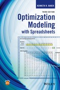
The product mix problem is a variation of the basic allocation model. It follows the structure of the allocation model by prescribing the maximization of profit contribution subject to LT constraints. Typically, the decision variables correspond to quantities of various products to include in a company’s product mix. The constraints are usually of two types: capacity constraints on production resources and demand constraints on potential sales. In Example 2.1, suppose that the company markets its chairs, desks, and tables through a distributor who also provides monthly forecasts of demands. Next month’s forecasts are as follows.
| Chairs | Desks | Tables | |
| Demand | 300 | 120 | 144 |
With this information, we can extend the basic allocation model to include three demand constraints as well. The full model takes the following algebraic form:

The spreadsheet version of this model simply adds three rows to the model in Figure 2.6. Most easily, the LHS formula can be copied from the wood supply constraint (cell E14) into cells E15:E17 after the new coefficients have been added, as shown in Figure 2.7.
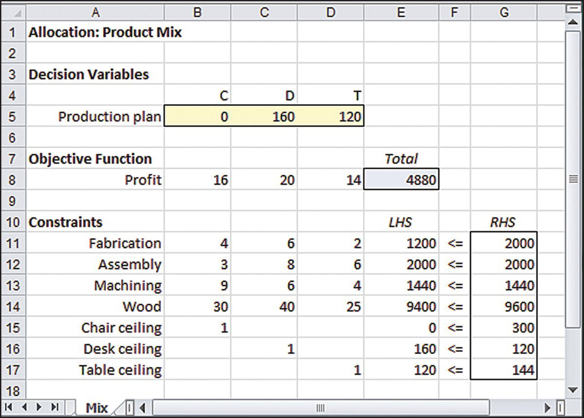
Figure 2.7 Product mix model.
We must then update the model specification so that all seven constraints are included. To make this adjustment, we can return to the Solver Parameters window, press the Add button, and append the constraints in rows 15–17 via the Add Constraint window.
Alternatively, to update the allocation model, we can select the existing entry in the Constraints window and press the Change button. Then, we can edit the entry so that the Constraints window displays only one set of constraints. It’s helpful to notice that the solution of 160 desks and 120 tables is not feasible in the expanded model because the newly added desk ceiling is violated.
A new optimization run then reveals that the optimal product mix becomes 16 chairs, 120 desks, and 144 tables, as shown in Figure 2.8. The optimal profit contribution in the product mix model is $4672. This amount is less than the optimal profit in the original allocation model. Not surprisingly, the imposition of demand ceilings leads to a reduction in the optimal profit. This outcome illustrates the intuitive principle that the addition of constraints to a model cannot improve the optimal objective function—it will be the same or worse when constraints are added.

Figure 2.8 Optimal solution to the product mix model.
Three binding constraints occur in the product mix model: the demand ceiling for desks, the demand ceiling for tables, and the machining capacity. None of the other constraints is binding.
2.3 COVERING MODELS
The covering problem calls for minimizing an objective (usually cost related) subject to GT constraints on required coverage. Whereas the allocation model divides resources and assigns them to competing activities, the covering model combines resources and coordinates activities. Consider the example of Herrick Foods Company.
To determine the decision variables, we again ask, “What must be decided?” The answer is we need to determine the amount of each ingredient to put in a package of trail mix. For the purposes of notation, we can use S, R, F, P, and W to represent the number of pounds of each ingredient in a package.
Next, we ask, “What measure will we use to compare sets of decision variables?” This should be the total cost of a package, and our interest lies in the lowest possible total cost. To calculate the total cost of a particular composition, we sum the costs of each ingredient in the package:
To identify the model’s constraints, we ask, “What restrictions limit our choice of decision variables?” In this scenario, the main limitation is the requirement to meet the specified nutritional profile. Each dimension of this profile gives rise to a separate constraint. An example of such a constraint states, in words, that the number of grams of vitamins provided in the package must be greater than or equal to the number of grams required by the specified profile. Laying out those words in the format of an inequality, we can write
where we chose to place “grams required” on the RHS because it is represented by a parameter of the model (16 grams in this case). Converting the inequality to symbols, we can then write
Similar constraints must hold for mineral, protein, and calorie content. The entire model, stated in algebraic terms, reads as follows:

In this basic scenario, no other constraints arise, although we could imagine that limits might exist on the quantities of the ingredients available, expressed as LT constraints, or a weight requirement for the package might exist, expressed as an EQ constraint.
A spreadsheet model for the basic scenario appears in Figure 2.9. Again, we see the three modules: a highlighted row for decision variables, a highlighted single cell for the objective function value, and a set of constraint relationships with highlighted RHS’s. If we were to display the formulas for this model, we would again see that the only formula in the worksheet is the SUMPRODUCT formula.

Figure 2.9 Model for Herrick Foods example.
Once we have persuaded ourselves that the model is valid, we proceed to the Solver Parameters window and enter the following information:

As in the allocation model, we check the box for nonnegative variables and select the linear solver.
After contemplating some hypotheses about the problem (e.g., will the solution require all five ingredients?) we run Solver and examine the Solver Results window, which conveys the optimality message. The optimal solution is reproduced in Figure 2.10. It calls for 0.48 pounds of seeds, 0.33 pounds of raisins, and 1.32 pounds of flakes, with no nuts at all. Evidently, nuts are prohibitively expensive, given the nature of the required nutritional profile and the other ingredients available. The optimal mix achieves all of the nutritional requirements at a minimum cost of $7.54. The tight constraints in this solution are the requirements for minerals, protein, and calories.

Figure 2.10 Optimal solution for the Herrick Foods model.
Herrick Foods might decide that trail mix without nuts is not an appealing product. This concern illustrates another situation where the solution to the model may not represent a solution to the practical problem. In building the model, we have not considered the implication of a product without nuts. Alerted to this possibility, we may wish to revisit the model and make sure that some nuts appear in the optimal mix. One way to do so is to require a minimum of 0.15 pounds of both pecans and walnuts in the mix. In Figure 2.11 displays an amended model that requires at least 0.15 pounds of every ingredient.

Figure 2.11 Herrick Foods model with additional constraints.
The value of 0.15 appears just below the corresponding decision variable, and in the Solver Parameters window, we add the constraint that the range B5:F5 must be greater than or equal to the range B6:F6. With this update, we obtain the following model specification:

The requirement that a particular decision variable must be greater than or equal to a given value is called a lower bound constraint. Here, the first set of constraints is formulated as a range of lower bound constraints. Similarly, a requirement that a particular decision variable must be less than or equal to a given value would be called an upper bound constraint. (We could have used such constraints in the product mix model, but in Figure 2.7, we posed them in the standard SUMPRODUCT style, so that they resembled the other constraints in the model.)
After including the lower bound constraints, running Solver again produces the optimal solution shown in Figure 2.12. By using linear programming and acknowledging a requirement to include all five ingredients in the ultimate mixture, Herrick Foods has identified the desired composition of its trail mix product.

Figure 2.12 Optimal solution to the modified Herrick Foods model.
Imposing lower bounds on the original Herrick Foods model leads to an optimal solution that contains all five of the ingredients. We might have expected that nuts would appear exactly at their lower limit because without the lower bound constraints, the optimization left nuts completely out of the solution. Thus, when we added the lower bound, there was no incentive to include nuts at any level greater than the lower bound. The optimal cost is also higher in the amended model than in the original, at $8.33. This result again reflects the intuitive principle that adding constraints to a model cannot improve the objective function—it will be the same or worse when constraints are added.
The trail mix example is a simplified version of a classic covering problem known as the diet problem. This problem arises, for example, in the determination of weekly menus for large institutional populations, such as those in summer camps, nursing homes, and prisons. The purpose of the model is to determine meal selection for each of the 21 meals served each week to everyone in a large group. The variables may represent quantities of various food groups (meats, vegetables, fruits, etc.), and weekly nutritional requirements reflect limits on the totals of weekly requirements for fat, calories, protein, carbohydrates, and so on. A common phenomenon, akin to the results of our first trail mix model, is that cost minimization drives the solution toward a limited number of meals. Campers may not find a steady diet of tofu appealing, even if that is the model’s optimal solution. Subtle differences between the problem and the model become clearer once a solution is obtained. For that reason, a more detailed and complicated set of constraints must often be added to the diet model in order to generate an appetizing weekly menu.
2.3.1 The Staff-Scheduling Problem
Many service industries face the problem of scheduling their workforce to meet fluctuating staffing requirements. Nurses, telephone operators, toll collectors, and bus drivers operate in this type of environment—providing service over a period that extends beyond the normal 8-hour working day and possibly continuing around the clock. Many companies restrict themselves to full-time workers, and they meet fluctuating requirements of this sort by assigning staff to overlapping work shifts. As an example, consider the daily staffing problem at Acme Communications.
For Acme’s problem, the decision variables are the number of operators assigned to each of the six starting times. For example, let x1 represent the number assigned to begin work on shift #1. These operators work during shifts #1 and #2, from 2 am to 10 am. Similarly, x2 represents the number assigned to work during shifts #2 and #3, from 6 am to 2 pm. With this notation, the number of operators working during shift #2 must equal x1 + x2; by a similar logic, the number of operators working during shift #3 must equal x2 + x3; and so on. Finally, the number working during shift #1 must equal x6 + x1 because the requirements repeat in 24-hour cycles. An algebraic statement of the problem is shown below:

Figure 2.13 shows a spreadsheet model for this problem.

Figure 2.13 Staffing model.
Staffing models of this sort have a distinctive structure. First, because the number of operators working on any given shift is the total assigned to two starting times, two variables appear in each constraint. Thus, in the spreadsheet, there are two 1’s on the LHS of each constraint row. Second, because operators work two consecutive shifts, two consecutive 1’s appear in the columns corresponding to variables. (In the case of x6, shifts #6 and #1 are consecutive.) The model specification is as follows:

Figure 2.13 displays an optimal solution, which achieves a total workforce of 105 by assigning various numbers of operators to five starting times, with no one starting work at 10 pm.
In general, we can structure the staff-scheduling model around the shift definition. Time periods correspond to rows in the model and alternative shift assignments correspond to columns. For a problem in which the assignments correspond to days, we can imagine seven constraints (each one representing a daily staffing requirement) and seven assignments (each one corresponding to a different start of a 5-day work stretch). In the constraints module, the column of coefficients under a given shift assignment shows the profile of the work shift. In Figure 2.13, those coefficients are two consecutive 1’s, reflecting the fact that each assignment comprises two consecutive 4-hour time periods. In a more detailed version with 2-hour time periods, we can imagine four consecutive 1’s. In an hourly version, we can imagine eight consecutive 1’s. In most applications, however, when the time periods are this detailed, provisions are usually made for meal breaks as well. As an example, imagine a service facility that operates over a 12-hour span from 6 am to 6 pm. Shifts begin on the hour and contain 8 hours of work with an hour break in the middle. In this case, the columns of the model would appear as follows.
| Start | 6 am | 7 am | 8 am | 9 am | |||||||
| 1 | 0 | 0 | 0 | 6−7 | Requirements | ||||||
| 1 | 1 | 0 | 0 | 7−8 | Requirements | ||||||
| 1 | 1 | 1 | 0 | 8−9 | Requirements | ||||||
| 1 | 1 | 1 | 1 | 9−10 | Requirements | ||||||
| 0 | 1 | 1 | 1 | 10−11 | Requirements | ||||||
| 1 | 0 | 1 | 1 | 11−12 | Requirements | ||||||
| 1 | 1 | 0 | 1 | 12−1 | Requirements | ||||||
| 1 | 1 | 1 | 0 | 1−2 | Requirements | ||||||
| 1 | 1 | 1 | 1 | 2−3 | Requirements | ||||||
| 0 | 1 | 1 | 1 | 3−4 | Requirements | ||||||
| 0 | 0 | 1 | 1 | 4−5 | Requirements | ||||||
| 0 | 0 | 0 | 1 | 5−6 | Requirements | ||||||
For the particular set of hourly staff requirements shown in Figure 2.14, the optimal staff size is 57.

Figure 2.14 Hourly staffing model.
However, if work rules allow the lunch break to occur after as few as 3 hours of work or as many as 5 hours of work, then 12 full-time shift assignments are available, rather than four. The shift start times would remain the same, but the column profiles would take the following form.
| Start | 6 | 6 | 6 | 7 | 7 | 7 | 8 | 8 | 8 | 9 | 9 | 9 |
| 1 | 1 | 1 | 0 | 0 | 0 | 0 | 0 | 0 | 0 | 0 | 0 | |
| 1 | 1 | 1 | 1 | 1 | 1 | 0 | 0 | 0 | 0 | 0 | 0 | |
| 1 | 1 | 1 | 1 | 1 | 1 | 1 | 1 | 1 | 0 | 0 | 0 | |
| 0 | 1 | 1 | 1 | 1 | 1 | 1 | 1 | 1 | 1 | 1 | 1 | |
| 1 | 0 | 1 | 0 | 1 | 1 | 1 | 1 | 1 | 1 | 1 | 1 | |
| 1 | 1 | 0 | 1 | 0 | 1 | 0 | 1 | 1 | 1 | 1 | 1 | |
| 1 | 1 | 1 | 1 | 1 | 0 | 1 | 0 | 1 | 0 | 1 | 1 | |
| 1 | 1 | 1 | 1 | 1 | 1 | 1 | 1 | 0 | 1 | 0 | 1 | |
| 1 | 1 | 1 | 1 | 1 | 1 | 1 | 1 | 1 | 1 | 1 | 0 | |
| 0 | 0 | 0 | 1 | 1 | 1 | 1 | 1 | 1 | 1 | 1 | 1 | |
| 0 | 0 | 0 | 0 | 0 | 0 | 1 | 1 | 1 | 1 | 1 | 1 | |
| 0 | 0 | 0 | 0 | 0 | 0 | 0 | 0 | 0 | 1 | 1 | 1 |
With these rules in place, the optimal staff size drops to 54. The example illustrates how an “optimal” solution can disguise possible inefficiency until we view the problem from a broader perspective. The solution in the four-shift model of Figure 2.14 is optimal for the situation it describes, but the rigidity of the rules governing shift patterns leads to inefficiency. When these rules become more flexible, then a more efficient solution is attainable. In contrast to the effect of additional constraints, additional flexibility can improve the objective function. Nevertheless, a good deal of overstaffing occurs in either model. We might have to look beyond the optimization model to avoid some of this remaining inefficiency. For example, if we can create incentives that a shift customer demands from one period to another, we can influence the size of the optimal staff.
One variation of the staff-scheduling problem combines full- and part-time shifts. We can imagine full-time shifts as columns in which the 1’s delineate an 8-hour workday, whereas the part-time shifts might be columns containing a smaller number of 1’s. Such models usually have an objective function that measures the cost of the workforce rather than its size to reflect salary differences between full- and part-time workers. In all these variations, however, the essential structure of the model represents a covering problem by minimizing workforce cost or workforce size subject to a systematic set of GT constraints for time-dependent staffing requirements.
2.4 BLENDING MODELS
Blending relationships are very common in linear programming applications, yet they remain difficult for beginners to identify in problem descriptions and to implement in spreadsheet models. Because of this difficulty, we begin with a special case—the representation of proportions. As an example, let’s return to the product mix version of Example 2.1. In Figure 2.8, the optimal product mix consisted of 16 chairs, 120 desks, and 144 tables. Suppose that this outcome is unacceptable because of the imbalance in volumes. For more balance, the marketing department might require that each product must make up at least 20% of the units sold.
When we describe outcomes in terms of a proportion and place a floor (or ceiling) on the proportion, we are using a special type of blending constraint. In our example, a direct statement of the requirement for chairs is the following:
This GT constraint has a parameter on the RHS and all the decision variables on the LHS, as is usually the case. Although this is a valid constraint, it is not in linear form because the quantities C, D, and T appear in both the numerator and denominator of the fraction. (The ratio divides decision variables by decision variables.) However, we can convert the nonlinear inequality to a linear one with a bit of algebra. First, multiply both sides of the inequality by (C + D + T), yielding
Next, we collect terms involving the decision variables on the LHS to obtain
This form conveys the same requirement as the original fractional constraint, and we recognize it immediately as a linear form. The coefficients on the LHS turn out to be either the complement of the 20% floor (1–0.2) or the floor itself (but with a minus sign). In a similar fashion, the requirement that the other products must respect the floor leads to the following two constraints:

Appending these three constraints to the product mix model gives rise to the linear program described in Figure 2.15. In the figure, we show the spreadsheet after the model has been optimized. Before the constraints were added, the optimal mix generated profits of $4672. With the 20% floor imposed, we expect optimal profits to drop. As shown in Figure 2.15, the new optimal mix becomes 48 chairs, 120 desks, and 72 tables. Thus, swapping chairs for tables in the product mix, we can achieve the best possible level of profit, achieving a total of $4176. As we might have expected, chairs make up exactly 20% of the optimal output in this solution, while desks and tables each account for more than 20%.

Figure 2.15 Modified product mix model.
Whenever we encounter a constraint in the form of a lower limit or an upper limit on a proportion, we can follow similar steps:
- Write the fraction that expresses the constrained proportion.
- Write the inequality implied by the lower limit or upper limit.
- Multiply through by the denominator and collect terms.
The result should be a linear inequality, ready to incorporate in the model.
In general, the blending problem involves mixing materials that have different individual properties and describing the properties of the blend with weighted averages. We might be familiar with the phenomenon of mixing from spending time in a chemistry laboratory mixing fluids with different concentrations of a particular substance, but the concept extends beyond laboratory work. Consider the example of Keogh Coffee Roasters.
For a little background on blending arithmetic, suppose that we blend Brazilian and Peruvian beans in equal quantities of 25 pounds each. Then we should expect the blend to have an aroma rating of 80, just halfway between the two pure ratings of 75 and 85. Mathematically, we take the weighted average of the two ratings:

Now, suppose that we blend the beans in amounts B, C, and P. The blend has an aroma rating calculated by a weighted average of the three ratings:

To impose a constraint that requires the aroma rating to be at least 78, we write
Once again, this constraint is nonlinear, by virtue of having decision variables in the numerator and denominator of the fraction. However, as shown previously, we can convert the requirement into a linear constraint. First, multiply both sides of the inequality by (B + C + P), yielding
Next, collect terms involving the decision variables on the LHS to obtain
This form conveys the same requirement as the original fractional constraint but in linear form. The coefficients on the LHS turn out to be just the differences between the individual aroma ratings (75, 60, 85) and the requirement of 78, with signs indicating whether the individual rating is above or below the target. In a similar fashion, a requirement that the strength of the blend must be at least 16 leads to the constraint
In general, the natural way to describe a blending requirement uses fractions, but in that form, blending requirements are nonlinear. We prefer to convert these requirements to linear constraints because with a linear model we can harness the full power of the linear solver. As we shall see later, the nonlinear solver has more limitations than the linear solver.
Now, with an idea of how to restate the blending requirements, we return to Example 2.4. In addition to the blending constraints, we need a constraint that generates a 4000-pound blend, along with three constraints that limit the supplies of the different beans. The algebraic problem statement is as follows:

Figure 2.16 shows the spreadsheet for our model, which contains a covering constraint and three allocation constraints, in addition to the two blending constraints. In a sense, the model has what we might think of as covering and allocation constraints, in addition to blending constraints. The Blending Data module, in rows 19–21, is not strictly part of the optimization model. We’ll come back to this part of the worksheet later. Each constraint in rows 11–16 is expressed in our standard form: a SUMPRODUCT formula on the LHS and a parameter on the RHS. This model contains three LT constraints and three GT constraints. It is helpful to keep constraints of the same type in adjacent locations on the worksheet, for convenience in entering the constraint information in the Solver Parameters window. In this case, with only two entries in the Constraints window, we can specify all six inequalities.

Figure 2.16 Keogh Coffee Roasters model.
The output constraint is formulated as an inequality. Although Keogh Coffee Roasters wishes to produce 4000 pounds, our model allows the production of a larger quantity if this will reduce costs. (Our intuition probably tells us that we should be able to minimize costs with a 4000-pound blend, but we would accept a solution that reduced costs while producing more than 4000 pounds: we could simply throw away the excess.) In many situations, it is a good idea to use the weaker form of the constraint, giving the model some “additional rope” and avoiding EQ constraints. In other words, we should build the model with some latitude in satisfying the constraints of the decision problem whenever possible. The solution will either confirm our intuition (as this one does) or else teach us a lesson about the limitations of our intuition.
The model specification is the following:

The linear solver produces an optimal blend of 1500 pounds of Brazilian, 520 pounds of Colombian, and 1980 pounds of Peruvian beans, for a total cost of $2448, as shown in the figure. By using linear programming, Keogh Coffee Roasters can optimize the cost of its blend while meeting its taste and aroma requirements. Of the two blending constraints, only the first (aroma) constraint is binding in this solution; the optimal blend actually has better-than-required strength. The output constraint is also binding (consistent with our intuitive expectation), as is the limit on Brazilian supply.
In Figure 2.16, we calculate the actual aroma and taste ratings in cells E19:E20, using the weighted average ratio formula directly. This module is added for convenience in the interpretation of the solution. It is not part of the Solver model in the sense that none of the cell addresses in the Solver Parameters window specifies cells in rows 19 or 20. For example, the calculation in cell E19 uses the formula =SUMPRODUCT($B$5:$D$5,B19:D19)/E13.
Whereas the first constraint of the model is binding (LHS and RHS of row 11 are both equal to zero), the aroma calculation in the Blending Data module shows that the weighted average equals the requirement of 78 exactly. Although the second constraint shows that the strength requirement is not binding, the comparison of LHS (4540) with RHS (zero) is not as helpful as a means of interpreting the slack in the constraint. However, cell E20 shows that the optimal blend’s strength is 17.14, which we can easily compare to the requirement of 16, giving us a sense of how much this blend exceeds the constraint.
Blending problems arise whenever weighted averages characterize the properties of a composite product. In our example, we treated taste and aroma as if they were numerically objective measures, for the purposes of illustration. However, it is not difficult to enumerate some applications where the parameters are “harder” numbers and blending concerns are relevant:
- Gasoline is a blend, and the octane rating of gasoline is a weighted average of its constituents. The inputs into a gasoline blend have different octane ratings as a function of their crude oil source and their previous processing steps. The classification of gasoline blends as regular, premium, or super premium is usually based on a minimum octane rating in each category. The principle of weighted average blending applies as well to other fluids, such as the viscosity of lubricants, the sugar content of fruit juice, or the fat content of ice cream.
- Chemical compounds other than fluids often have such constituents as nickel, copper, sulfur, potassium, and the like. These constituents may have functional benefits, or they may be considered impurities. In either event, different compounds have different percentage compositions of these elements, and compositions blend according to weighted averages when elements are mixed together. The principle of weighted averages applies to metal in alloys, pollutants in emissions, or active ingredients in medications.
- Investment portfolios consist of discrete assets such as stocks and bonds. Each asset in the portfolio has its own financial characteristics, but properties of the overall portfolio dictate admissible investment strategies. The principle of weighted averages applies to maturities of bonds, rates of return on stocks, and riskiness ratings of assets.
2.5 MODELING ERRORS IN LINEAR PROGRAMMING
We have presented our examples as if they were built by knowledgeable analysts, with each step implemented correctly and all errors avoided. However, someone new to the experience of building optimization models seldom makes it through all of the steps without some kind of difficulty. Even experts run into problems, especially when they are working on complex models. It is probably unrealistic to expect that the process of building and analyzing a model can be carried out without encountering some sort of difficulty along the way. To be effective in modeling, we have to know how to deal with errors when they occur.
2.5.1 Exceptions
Given a linear programming model, Solver always finds an optimal solution, provided one exists. The first kind of modeling error is formulating a model that does not have an optimal solution. Two exceptions can cause difficulties: infeasible constraints and an unbounded objective function.
A model contains infeasible constraints if no set of decision variables can satisfy all constraints simultaneously. For example, in the product mix example of Figure 2.8, suppose we had signed a contract promising that 200 chairs would be delivered to a single large customer, as part of the product mix. Adding the requirement C ≥ 200 to the other constraints of the model creates an inconsistency. (The implied machining requirement would be 1800 hours, which exceeds the capacity available.) Presented with a set of inconsistent constraints, Solver detects the inconsistency and delivers the following message in the Solver Results window:
Solver could not find a feasible solution.
Whenever this message appears, there must have been an inconsistency in the set of constraints.
For the model builder, the task is to locate the inconsistency when confronted with the infeasibility message. There are potentially two levels to this task: (1) finding the offending constraint or constraints and (2) identifying the source of the inconsistency. Sometimes, the offending constraint can be discovered by “eyeballing” the model—scanning for visual clues to the location of an error. For example, a parameter could be entered incorrectly. (Perhaps, the chair contract calls for only 20 units, but 200 have been entered inadvertently.) Alternatively, a constraint could be entered backward, as an LT constraint when it should have been a GT constraint. However, the more standard way to search for an inconsistency is to remove constraints from the model, one at a time, and to rerun Solver each time. (In large problems, it might make more sense to remove several constraints at a time.) If the model remains infeasible, restore the constraint and try removing a different one. If the model reaches an optimal solution, then we know that something about the constraint we removed was a partial cause of the infeasibility.
Identifying the source of an inconsistency refers to the part of the task that lies at the interface between model and problem. If the inconsistency resulted from a typo, then it is a simple matter to repair it. However, a more subtle difficulty arises when the formulation contains too many constraints. This result can occur if, during the modeling process, a thorough attempt is made to include all the considerations mentioned by various parties. Isolated desires and secondary considerations could wind up being expressed as model constraints, contributing to a logical conflict. In these situations, it makes sense to eliminate some of the constraints, so the model is at least feasible. Thereafter, various additional considerations can be revisited to see whether they can be accommodated without causing infeasibility.
The second kind of modeling error occurs when there is no limit to the objective function in the direction of optimization. An unbounded objective function occurs if, with a set of feasible decisions, the objective can grow infinitely positive in a maximization problem or infinitely negative in a minimization problem. The most common cause of an unbounded objective is failure to require nonnegative values for the decision variables. For example, in the trail mix example of Figure 2.10, suppose we had forgotten to require nonnegativity. Then it would be mathematically possible to make the objective function as negative as we wish by taking negative quantities for some of the ingredients. Consider the mix corresponding to R = 115, P = −40, and W = −50. This combination satisfies all four constraints, with a total cost of −$5.00. Mathematically, this mix could be expanded in the same proportion, with all constraints met and the total cost becoming as negative as we like. Presented with conditions that permit an objective function to expand infinitely in the direction of optimization, Solver detects the unbounded possibilities and delivers the following result message in the Solver Results window:
The objective (Set Cell) values do not converge.
The reference to “Set Cell” provides consistency with older versions of the software, which did not use the term “objective.”
For the model builder, the task is to locate the cause of an unbounded objective function. The problem could lie in the objective function or in the constraints. A simple typo in an objective function cell could induce unbounded possibilities. However, unboundedness can also occur when a constraint is omitted from the model, allowing decision variables to reach values never intended by the model builder. Whereas locating the cause of infeasibility directs attention to the constraints, it is more difficult to know where to look for the cause of unboundedness.
2.5.2 Debugging
Even a model that contains feasible constraints and a bounded objective function can be logically flawed. Beyond its ability to detect infeasible and unbounded formulations, Solver has no automatic means of detecting logical errors. That responsibility lies with the model builder. However, a few techniques that are helpful to spreadsheet users can augment the capabilities in Solver:
- Set all decision variables to zero. A good first step is to enter zero for each of the decision variables and confirm that the objective function and constraints behave as expected. Then, make one variable at a time positive. Taking successive values for a variable equal to 1, 10, and 100 can show whether the scaling properties of the model seem valid.
- Display formulas. By simultaneously pressing the Control and tilde (~) keys, we can look at all the formulas in the spreadsheet window. As in Figure 2.2, we look for the SUMPRODUCT formulas in the cells corresponding to the objective function and the LHS of each constraint. No other formulas are necessary, although in the next chapter we shall look at some cases where an alternative form is convenient. Pressing the Control and tilde keys simultaneously once more restores the display.
- Invoke Formula Auditing. The Formula Auditing tools appear on the Formulas tab in Excel. In Figure 2.17, we have selected, one at a time, each of the constraint formulas and clicked on the Trace Precedents icon for each one. The resulting logical map exhibits a systematic structure that helps validate the formulas. An asymmetric set of precedence arrows might suggest where a logical error can be found.
- Invoke the Cell Edit function. Selecting a formula cell and pressing the function key F2 can implement a similar kind of validation. The Cell Edit function displays a color-coded interpretation of the formula, highlighting its constituent cells. In linear programming models, this kind of verification might catch a formula in which the range was entered or pasted incorrectly.
- Use the Change Constraint option. Another way to verify that ranges are correctly entered involves the Change Constraint window. In the Solver Parameters window, select an entry in the Constraints window and press the Change button. Then the LHS’s of the selected constraints are highlighted in the model when the Change Constraint window appears. This step can sometimes detect an error in specifying the location of a constraint, especially in complicated models where constraints might be arranged separately, at different locations on the worksheet.

Figure 2.17 Formula Auditing with the trace precedence command.
2.5.3 Logic
In Chapter 1, we pointed out the distinction between the convergence message and the optimality message in finding an optimal solution with the nonlinear solver. When we use the linear solver, that distinction does not arise. If we formulate a model that is feasible and bounded and if we use the linear solver, then the optimality message appears every time; we do not need to rerun Solver.
SUMMARY
This chapter has introduced three classes of linear programming models: allocation, covering, and blending. To some extent, these elementary models allow us to discuss the basic scenarios that lend themselves to linear programming models, so allocation, covering, and blending models might well be taken as the “ABC” of model building with linear programming. Allocation, covering, and blending models are also important building blocks for more complex models because many practical applications are combinations of these structures.
Linearity in both the objective function and constraints is the key structural assumption in linear programming. In the process of building a linear programming model, it is desirable to revisit the requirements of proportionality, additivity, and divisibility to confirm that their properties apply. Another less prominent assumption is the presumption of certainty in the elements of a linear programming model. Most of the time, linear programs are applied in situations where uncertainty can be suppressed without undermining the value of the model. Nevertheless, advanced forms of linear programming extend to situations where the uncertainty cannot be avoided.
Classification of linear programming models provides some immediate benefits. When we are trying to understand someone else’s model, our ability to classify may help us appreciate either the overall structure of a model or some of its major parts. Also, when we are trying to develop a model from scratch, we can accelerate the process if we can classify the model or at least one portion of it. Model building requires that we recognize situations that lend themselves to representation in a model. Familiarity with the elementary scenarios that go with allocation, covering, and blending helps us to recognize structure in an actual situation. Finally, when we are debugging our own model, classification allows us to compare what we have built with the standard template. That comparison helps us to detect mistakes we may have made in constraint coefficients and constants or perhaps even in objective function coefficients. Also included in this chapter were a number of suggestions for debugging that apply throughout the remainder of the book.
The classification of linear programs is not as precise as, say, biological classification. Moreover, as we saw in Example 2.4, a linear program can combine types. Although we will encounter additional classes of models in the next three chapters, we will not attempt to classify every possible linear program. Instead, the purpose is to appreciate the kinds of situations that lend themselves well to linear programming. Then, when we encounter similar situations in the world around us, we’ll be able to think about those situations in terms of a corresponding linear programming structure. Armed with knowledge of these building blocks, we can analyze new situations by recognizing familiar structures within them, thus identifying some of the important elements (variables and constraints) of the eventual model.
EXERCISES
- 2.1 Verifying Linearity: Revisit Examples 2.2, 2.3, and 2.4 and verify that the properties of proportionality, additivity, and divisibility are reasonable assumptions in modeling each problem.
- 2.2 Allocating Ingredients: The Pizza Man is a local shop that plans to make all of its sales this Saturday from its sidewalk tables during the town’s holiday parade. On this occasion, the shop’s owners know that customers will buy by the slice and any kind of pizza offered will sell. The Pizza Man offers plain, meat, vegetable, and supreme pizzas. Each variety has its own requirement for sauce, cheese, dough, and toppings (in ounces, as shown in the table), and each has its own selling price.
Plain Meat Vegetable Supreme Available Dough 5 5 5 5 200 Sauce 3 3 3 3 90 Cheese 4 3 3 4 120 Meat 0 3 0 2 75 Vegetables 0 0 3 2 40 Price $8 $10 $12 $15 The Pizza Man expects to use its entire stock of ingredients and wishes to maximize revenue from its sales.
- What mix of pizzas should be made? (Assume that fractions can be sold.)
- What is the maximum sales revenue?
- Which ingredients are economically scarce (which ones limit profits)?
- 2.3 Workforce Scheduling: The operations manager at Metropolis National Bank has a staffing problem. Demand for clerical staff varies throughout the day, but 24-hour coverage is necessary because the bank handles a number of international transactions. A recent study has shown how many clerical workers are needed each hour in the course of the day, as shown below. (Hour 1 is from midnight to 1 am.)
Hour 1 2 3 4 5 6 7 8 9 10 11 12 Staff 4 3 2 2 3 5 6 6 9 10 10 10 Hour 13 14 15 16 17 18 19 20 21 22 23 24 Staff 12 12 8 6 7 7 7 6 5 4 4 4 Under current labor policies, clerical workers may be assigned to any one of six shifts, some of which overlap. The shifts and salary costs are as follows.
Shift Daily Cost ($) 2 am–10 am 160 6 am–2 pm 145 10 am–6 pm 148 2 pm–10 pm 154 6 pm–2 am 156 10 pm–6 am 160 - Provide the operations manager with a schedule that will deploy enough staff to meet the hourly requirements at the minimum daily total cost.
- In the optimal schedule, how many hourly periods are overstaffed?
- 2.4 Selecting a Portfolio: A portfolio manager has developed a list of six investment alternatives for a multiyear horizon. These are Treasury bills, Common stock, Corporate bonds, Real estate, Growth funds, and Savings and loans. These investments and their various financial factors are described below. In the table, the return is given as an annual percentage, and the length represents the estimated number of years required for the annual return to be realized. The risk coefficient is a subjective estimate representing the manager’s appraisal of the relative safety of each alternative, on a scale of 1–10. The growth potential is an estimate of the potential increase in value over the horizon.
Portfolio Data Alternative TB CS CB RE GF SL Length (years) 4 7 8 6 10 5 Annual return (%) 6 15 12 24 18 9 Risk coefficient 1 5 4 8 6 3 Growth potential (%) 0 18 10 32 20 7 The manager wishes to maximize the return on a $3 million portfolio, subject to the following restrictions:
- The weighted average length should not exceed 7 years.
- The weighted average risk coefficient should not exceed five.
- The weighted average growth potential should be at least 10%.
- The investment in real estate should be no more than twice the investment in stocks and bonds (i.e., in CS, CB, and GF) combined.
- What are the optimal return and the optimal allocation of investment funds? (Give the optimal return in dollars and also as a percentage.)
- What is the marginal rate of return? In other words, what would be the return on the next dollar invested if there were one more dollar in the portfolio?
- For additional investment beyond the original $3 million, how does the optimal allocation change?
- 2.5 Oil Blending: An oil company produces three brands of oil: regular, multigrade, and supreme. Each brand of oil is composed of one or more of four crude stocks, each having a different lubrication index. The relevant data concerning the crude stocks are as follows.
Crude Stock Lubrication Index Cost ($/Barrel) Daily Supply (Barrels) 1 20 7.1 1000 2 40 8.5 1100 3 30 7.7 1200 4 55 9 1100 Each brand of oil must meet a minimum standard for a lubrication index, and each brand thus sells at a different price. The relevant data concerning the three brands of oil are as follows.
Brand Minimum Lubrication Index Selling Price ($/Barrel) Daily Demand (Barrels) Regular 25 8.5 2000 Multigrade 35 9 1500 Supreme 50 10 750 The task is to determine an optimal output plan for a single day, assuming that production can be either sold or else stored at negligible cost. The daily demand figures are subject to alternative interpretations. Investigate the following.
- The daily demands represent potential sales. In other words, the model should contain demand ceilings (upper limits). What is the optimal profit?
- The daily demands are strict obligations. In other words, the model should contain demand constraints that are met precisely. What is the optimal profit?
- The daily demands represent minimum sales commitments, but all output can be sold. In other words, the model should permit production to exceed the daily commitments. What is the optimal profit?
- 2.6 Coffee Blending and Sales: Hill-O-Beans Coffee Company blends four component beans into three final blends of coffee: one is sold to luxury hotels, another to restaurants, and the third to supermarkets for store-label brands. The company has four reliable bean supplies: Argentine Abundo, Peruvian Colmado, Brazilian Maximo, and Chilean Saboro. The table below summarizes the very precise recipes for the final coffee blends, the cost and weekly availability information for the four components, and the wholesale price per pound of the final blends. The percentages indicate the fraction of each component to be used in each blend.
Component Hotel Restaurant Market Cost per Pound ($) Pounds Available Abundo 20% 35% 10% 0.60 40,000 Colmado 40% 15% 35% 0.80 25,000 Maximo 15% 20% 40% 0.55 20,000 Saboro 25% 30% 15% 0.70 45,000 Wholesale price per pound $1.25 $1.50 $1.40 The processor’s plant can handle no more than 100,000 pounds per week, and Hill-O-Beans would like to operate at capacity, if possible. Selling the final blends is not a problem, although the marketing department requires minimum production levels of 10,000, 25,000, and 30,000 pounds, respectively, for the hotel, restaurant, and market blends.
- To maximize weekly profit, how many pounds of each component should be purchased?
- How would the optimal profit change if there were a 1000-pound increase in the availability of Abundo beans? Colmado? Maximo? Saboro?
- 2.7 Production Planning for Automobiles: The Auto Company of America (ACA) produces four types of cars: subcompact, compact, intermediate, and luxury. ACA also produces trucks and vans. Vendor capacities limit total production capacity to at most 1,200,000 vehicles per year. Subcompacts and compacts are built together in a facility with a total annual capacity of 620,000 cars. Intermediate and luxury cars are produced in another facility with capacity of 400,000; and the truck/van facility has a capacity of 275,000. ACA’s marketing strategy requires that subcompacts and compacts must constitute at least half of the product mix for the four car types. Profit margins, market potential, and fuel efficiencies are summarized below.
Type Profit Margin ($/Vehicle) Potential Sales (in 000 s) Fuel Efficiency (MPG) Subcompact 150 600 40 Compact 225 400 34 Intermediate 250 300 15 Luxury 500 225 12 Truck 400 325 20 Van 200 100 25 The Corporate Average Fuel Efficiency (CAFE) standards require an average fleet fuel efficiency of at least 27 MPG. ACA would like to use a linear programming model to understand the implications of government and corporate policies on its production plans.
- What is the optimal annual profit for ACA?
- How much would the annual profit drop if the fuel efficiency requirement were raised to 28 MPG?
- 2.8 Make or Buy: A sudden increase in the demand for smoke detectors has left Acme Alarms with insufficient capacity to meet demand. The company has seen monthly demand for its electronic and battery-operated detectors rise to 20,000 and 10,000, respectively, and Acme wishes to continue meeting demand. Acme’s production process involves three departments: fabrication, assembly, and shipping. The relevant quantitative data on production and prices are summarized below.
Department Monthly Hours Available Hours/Unit (Electronic) Hours/Unit (Battery) Fabrication 2000 0.15 0.10 Assembly 4200 0.20 0.20 Shipping 2500 0.10 0.15 Variable cost/unit $18.80 $16.00 Retail price $29.50 $28.00 The company also has the option to obtain additional units from a subcontractor, who has offered to supply up to 20,000 units per month in any combination of electronic and battery-operated models, at a charge of $21.50 per unit. For this price, the subcontractor will test and ship its models directly to the retailers without using Acme’s production process.
- What are the maximum profit and the corresponding make/buy levels? (This is a planning model, and fractional decisions are acceptable.)
- Trace the effects of increasing fabrication capacity by 10%. How will the optimal make/buy mix change? How will the optimal profit change?
- 2.9 Leasing Warehouse Space: Cox Cable Company needs to lease warehouse storage space for 5 months at the start of the year. It knows how much space will be required in each month, and it can purchase a variety of lease contracts to meet these needs. For example, it can purchase 1-month leases in each month from January to May. It can also purchase 2-month leases in January through April, 3-month leases in January through March, 4-month leases in January and February, or a 5-month lease in January. In total, there are 15 possible leases it could use. It must decide which leases to purchase and how many square feet to purchase on each lease.
Since the space requirements differ month to month, it may be economical to lease only the amount needed each month on a month-by-month basis. On the other hand, the monthly cost for leasing space for additional months is much less than for the first month, so it may be desirable to lease the maximum amount needed for the entire 5 months. Another option is the intermediate approach of changing the total amount of space leased (by adding a new lease and/or having an old lease expire) at least once but not every month. Two or more leases for different terms can begin at the same time.
The space requirements (in square feet) and the leasing costs (in dollars per thousand square feet) are given in the two tables below.
Month January February March April May Requirements 15,000 10,000 20,000 5,000 25,000 Lease length 1 month 2 months 3 months 4 months 5 months Lease cost 280 450 600 730 820 The task is to find a leasing schedule that provides the necessary amounts of space at the minimum cost.
- Determine the optimal leasing schedule and the optimal total cost.
- Trace the effects of increasing the space required for January. How will the leasing schedule change? How will the total cost change?
- 2.10 Scheduling Tire Production: The Seaboch Tire Company produces four lines of tires: the economy, the glass-belted, the snow, and the radial tire. The problem it faces is to schedule two shifts of production during the last quarter of the calendar year. The production process primarily involves the use of vulcanization, fabrication, and plastometer equipment, but the limiting resource is the availability of the vulcanization machines. The four tires require different amounts of time at vulcanization, as tabulated below.
Tire Econ. Glass Snow Radial Hours/tire 4.5 5 5.5 6 A sales forecast is available, breaking down predicted sales (in thousands) by tire type and by month.
Sales October November December Econ. 8 7 6 Glass 18 16 18 Snow 4 15 15 Radial 6 5 8 In addition, the number of hours of vulcanizing time (in thousands), for each shift and for each month, is also known.
October October November November December December Shift 1 2 1 2 1 2 Hours 110 100 130 120 120 115 The labor cost of operating the vulcanizing machines is $10 per hour during the first shift and $12 per hour during the second shift. The other relevant cost is storage: It costs $4 per month for storage and handling at the warehouse, regardless of tire type. This cost is incurred when production is scheduled in advance of demand to ensure that demand is met on time.
- What production plan will minimize cost and meet demand at Seaboch Tire?
- How would the solution in (a) change if sales for each tire in December were 10% higher?