3
LINEAR PROGRAMMING: NETWORK MODELS
In the previous chapter, we examined allocation, covering, and blending models—three basic structures frequently encountered in linear programming applications. A fourth common structure is the network model, and we devote a separate chapter to it because of its distinctive nature. The network model describes configurations of flow in a connected system, where the flow might involve material, or people, or funds, etc. These configurations are conveniently described with flow diagrams, which help in the development of valid spreadsheet models. The possibility of doing some of the model building with a diagram makes network models a special category of linear programs.
The flow diagram is a modeling tool in its own right, and we can use it as a visual aid or an auditing device. Used as a visual aid, the flow diagram is an accessory, providing a picture of the problem structure to assist us in our main task, which is developing the spreadsheet representation of the linear program. In this role, the flow diagram is a preliminary step; it helps us build the spreadsheet model, and once we’ve done that, we may no longer need the diagram. Alternatively, used as an auditing device, the flow diagram allows us to translate a network picture directly into an algebraic formulation and vice versa. This approach integrates the flow diagram with the spreadsheet model. In this role, the diagram allows us to develop a model on two fronts simultaneously, and we can use the diagram to check for errors and omissions as we build the spreadsheet model.
In terms of the optimization software, no new features are needed to deal with network models. Therefore, the software features covered in the previous chapter are sufficient for this chapter as well.
We first study three types of special network problems that illustrate the use of flow diagrams as visual aids. The distinguishing feature of special network models is an inherent from/to flow pattern that lends itself to the row-and-column format of the spreadsheet. We then move on to general network problems involving other flow patterns, where we illustrate how to integrate the flow diagram with the development of a spreadsheet. As we will see, the distinguishing feature of network models is a basic conservation law governing patterns of flow. This feature allows us to identify the key constraints needed for the model. In the course of this chapter, we encounter several applications of the conservation law, and we pay particular attention to the use of flow diagrams in modeling.
3.1 THE TRANSPORTATION MODEL
A central feature of physical supply chains is the movement of product from one or more source locations to a set of destinations where demand occurs. The cost of moving units of product, together with the cost of making the product, accounts for most of the cost of getting products to market. Small wonder, then, that a great deal of attention is paid to controlling the costs that occur in supply chains. The building block for performing this type of analysis is the transportation model. Consider the example of Goodwin Manufacturing.
Figure 3.1 displays a flow diagram showing the possible routes. In the diagram, the letters on the left designate the manufacturing plants, which supply the product. The letters on the right stand for the warehouses, where the demands occur. In this case, all supply–demand pairs represent potential shipping routes.

Figure 3.1 Flow diagram for Example 3.1.
Network terminology refers to flow along arcs or arrows in the diagram. Each arc connects two nodes or circles, and the direction of the corresponding arrow indicates the direction of flow. This flow incurs a cost: The unit cost of flow from any plant to any warehouse is given in Example 3.1. The flows along each of the 12 possible routes constitute the decision variables in the model. Although the diagram does not contain labels for the arcs, it would be natural to use the notation MA for the quantity shipped on the route from Minneapolis to Atlanta, MB for the quantity shipped on the route from Minneapolis to Boston, and so on.
This is an instance of the classical transportation problem, which is described by a set of sources and their supplies, a set of destinations and their demands, and the unit cost associated with each source–destination pair. In Example 3.1, the supplies are plant capacities—figures that would be provided by the production or manufacturing function. The demands are customer orders, typically marketing forecasts of near-term requirements, although they could be firm orders in environments where delivery lead times are relatively long. Unit costs are actual costs incurred internally, and they would be estimated from historical data in logistics records. If some of the potential routes had not been in use, the cost on those routes would have to be estimated by knowledgeable people in the distribution or transportation functions. Alternatively, the unit costs could arise as prices set by third parties who take responsibility for transportation of physical goods. In such cases, unit costs would be based on published rates for delivery by truck, rail, or air.
Figure 3.2 displays a spreadsheet model for the example, reflecting the distinctive from/to structure in the table describing the parameters of the problem. This structure lends itself readily to a row-and-column format, which is the essence of spreadsheet layout. Here, we adopt a convention that associates sources with rows and destinations with columns. In other words, flow moves conceptually in the spreadsheet from rows to columns. Because of this structure, it is helpful to depart from the standard linear programming layout used in Chapter 2 and to adopt a special format for this type of model. In particular, we can construct a spreadsheet model in rows and columns to mirror the table of parameters given in Example 3.1. In the Parameters module of the spreadsheet, we see all of the given information, displayed in an array. In the Decisions module, the decision variables (shaded for highlighting) appear in an array of the same size. At the right of each row is the “Sent” quantity, which is simply the sum of the flows along the row. Below each column of the array is the “Received” quantity, which is the sum in the column. The objective function, which is expressed as a SUMPRODUCT function in cell C18, is the total transportation cost for the system. It is the SUMPRODUCT of the two ranges, C5:F7 and C12:F14, that hold the unit cost parameters and the shipment decisions. In algebraic form, the objective function can be expressed as

Figure 3.2 Spreadsheet model for Example 3.1.
The transportation model has two kinds of constraints: LT supply constraints and GT demand constraints. For the Minneapolis plant, the amount shipped from Minneapolis must not exceed the Minneapolis capacity. In symbols, we can write the capacity constraint as
For Pittsburgh and Tucson, we have similar constraints:

Given the spreadsheet layout, these three constraints constitute a set of LT constraints that say Sent ≤ Capacity, or G12:G14 must be less than or equal to G5:G7. The left-hand side (LHS) of these constraints simply adds the outbound shipment quantities from a given location. For that reason, we don’t need to use a SUMPRODUCT formula in the worksheet; we can use the simpler SUM formula. Thus, as the display of formulas in Figure 3.3 demonstrates, the spreadsheet model uses both the SUMPRODUCT and SUM functions.

Figure 3.3 Formulas in the spreadsheet for Example 3.1.
For the Atlanta warehouse, the demand constraint requires that the amount received at Atlanta (from all sources) must be at least as large as the Atlanta demand. As we saw in Chapter 2, it is good practice to use the inequality form of this type of constraint, even though our intuition may tell us that there is no reason to ship more to Atlanta than is demanded. In symbols, this constraint reads
Similarly, for the other three warehouses, the constraints become

In the spreadsheet, these four constraints constitute a set of GT constraints that say Received ≥ Demand, or C15:F15 must be greater than or equal to C8:F8. Again, the LHS of these constraints can easily be expressed using the SUM formula. In the Solver Parameters window, we specify the model as follows.

As usual for linear programs, we select the Simplex LP solving method and check the box to make all variables nonnegative. This will be standard operating procedure when we are solving linear programs, so we won’t mention it specifically from now on, unless there is an exception.
The optimal solution, shown in Figure 3.2, achieves the minimum cost of $13,830. All demand constraints in this solution are binding, even though we permitted the model to send more than the requirement to each warehouse. This result makes intuitive sense because shipping more than is required to any warehouse would merely incur excess cost. Once we understand why there is no incentive to exceed demand, we can anticipate that there will be some excess capacity in the solution. This property occurs because total capacity comes to 40,000 cartons, while total shipment volume comes to only 39,000, as confirmed in cell G15. In particular, capacity constraints are binding at Pittsburgh and Minneapolis, but an excess capacity of 1,000 cartons remains at Tucson.
The solution, shown on the original network diagram in Figure 3.4, may be surprising to someone who has not previously seen the transportation model. Although there are 12 possible shipment routes in the model, the optimal solution uses only six. The flexibility in having three possible sources for meeting each demand is not fully utilized. After a little further thought, this pattern makes sense because many of the unused routes are expensive. Nonetheless, the solution uses the TA route, on which the unit cost is $0.65, and avoids the PC route, where the unit cost is $0.28. Such choices might be unexpected, but they reflect the systems view that an optimization model can take.

Figure 3.4 Optimal flows for Example 3.1.
As in other linear programming solutions, the transportation model provides both tactical and strategic information. If Goodwin Manufacturing had to implement a distribution plan immediately, then the plan shown in Figure 3.2 would be the cost-minimizing plan that its management seeks, representing the tactical interpretation of the model. However, if there is time to explore some changes in the given information, as strategic initiatives, then to reduce total transportation cost, Goodwin should explore ways of lowering one of the demand requirements or ways of adding capacity to Minneapolis or Pittsburgh because these actions loosen the binding constraints. At the margin, adding capacity at Tucson will not help in reducing total cost. Thus, by using linear programming to solve its transportation problem, Goodwin Manufacturing can determine the cheapest way to meet customer demands in the short run. It can identify some economically attractive strategic initiatives as well.
Example 3.1, which contains three sources and four destinations, shows how to build a suitable spreadsheet for the transportation problem. It is straightforward to adapt the spreadsheet design to any number of sources and any number of destinations. Again, the key formulation step is to display cost parameters and shipment quantities as separate arrays.
3.2 THE ASSIGNMENT MODEL
An important special case of the transportation problem has all capacities and all requirements equal to one. Moreover, the number of sources and the number of destinations are the same. This special case is known as the assignment problem. The one-to-one matching structure of an assignment is a practical problem. In addition, it arises as a portion of a more complicated model, as we shall see later. For the most part, we can set up and solve this special case in the same way that we dealt with the transportation problem. Consider the example of the Europa Auto Company.
We can think of an assignment as a selection of six numbers from the cost table, one from each row and one from each column. (Because the number of products is the same as the number of plants, we can think of either assigning plants to products or assigning products to plants.) The total cost associated with such an assignment is the sum of the numbers selected. This is merely another way of saying that the problem is a special transportation problem in which the row “capacities” are each one and the column “requirements” are also one. As such, we can construct a flow diagram to represent the decision problem in much the same way as in the transportation model of Figure 3.1. The diagram for the automaker example is shown in Figure 3.5, where each of the 36 arcs in the diagram represents a potential plant–product assignment.

Figure 3.5 Flow diagram for Example 3.2.
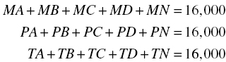
To construct the assignment model algebraically, we define our decision variables as the possible plant–product combinations, A1, A2,…, F6. Our objective function (denoted by z) is the total cost of an assignment, which can be expressed as the sum of 36 products. Each term in this sum is an assignment cost multiplied by a decision variable:
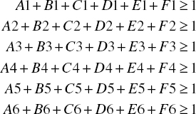
The decision variables must satisfy 12 constraints, 6 for the plants and 6 for the products. The row (plant) constraints restrict each plant to at most one product, as follows:

These constraints could also be written as equations. Meanwhile, the column (product) constraints ensure that each product has at least one source, as follows:
Again, these constraints could be written as equations without affecting the problem’s solution.
Alternatively, for a more compact algebraic representation, we can use xij to represent the assignment decisions. Specifically, xij = 1 if vehicle j is made at plant i. In addition, we let cij denote the cost of assigning plant i to vehicle j. The index i corresponds to a row number and the index j corresponds to a column number. Then, we can express the objective function—the system-wide cost of the assignment—as the following sum:
The constraints become

Because the assignment model is a special case of the transportation model with total capacity equal to total demand, we can be sure that the capacity and demand constraints will be binding. (This compact form of the problem statement will be useful to us in later chapters.)
The assignment problem is to minimize z subject to the 12 constraints on the variables. In neither of these formulations are there explicit considerations that would help us avoid fractional values for the decision variables. Although our problem statements allow the decision variables to be fractional, their optimal values will always be either zero or one, as we shall discuss later.
Figure 3.6 shows a spreadsheet model for the assignment problem. It resembles the spreadsheet for the transportation model introduced in Figure 3.2. The upper table contains a 6 × 6 array of assignment costs. The decisions are shown in the lower 6 × 6 table and highlighted. To the right of each row is the row sum and below each of the columns is the column sum. As in the transportation model (Fig. 3.2), these cells use the SUM formula. Finally, in cell B24, we highlight the value of the objective function, or total cost, which is computed as the SUMPRODUCT of the cost array and the decision array.

Figure 3.6 Spreadsheet model for Example 3.2.
Conceptually, each plant has a capacity of one (product) and each product has a requirement of one (plant), in analogy to the transportation model. Rather than include these parameters on the spreadsheet itself, they are entered as right-hand side (RHS) constants in the constraints. Normally, it is not good practice to enter RHS constants in the Solver Parameters window because we prefer to show parameters of the model on the spreadsheet itself, where we might want to explore some what-if questions. However, we make an exception here because the RHS will not change: Values of one represent the essence of the assignment problem. The specification of the model is as follows:

The LT constraints ensure that at most one product is assigned to each plant, and the GT constraints assure that each product has at least one plant assigned to it. (As mentioned earlier, we could also express all of the constraints as equations.)
Figure 3.6 displays the optimal solution, which achieves a minimum total cost of $314 million. This optimum is achieved by assigning the Sedan to Plant A, the Coupe to B, the SUV to C, the Van to D, the Truck to E, and the Compact to F. By solving this linear programming problem, Europa can find an economic assignment of vehicle models to plants, thus potentially saving millions of dollars over ad hoc assignment methods.
The assignment problem often arises when people must be assigned to tasks. The model assumes that quantitative scores apply to each person–task combination and the objective is to find a minimum (or maximum) total score. One classic application is the assignment of four swimmers to laps in a medley relay, where each lap corresponds to a different stroke and each swimmer has a lap time for each stroke. The assignment model has also been used to assign workers to shifts, courses to time slots, airline crews to flights, and purchase contracts to supplier bids. For our purposes in modeling, the assignment problem is simply a practical special case of the transportation problem.
3.3 THE TRANSSHIPMENT MODEL
The assignment problem turned out to be a simplified version of the transportation problem, specialized to unit demands at each destination and unit supplies at each source. By contrast, the transshipment problem is a complicated version of the transportation problem, containing two stages of flow instead of just one. In Figure 3.1—our diagram for the transportation problem—the system contains two levels (plants and warehouses), and all the flow takes place in one stage, from plants to warehouses. In many logistics systems, however, there are three major levels: plants, distribution centers (DCs), and warehouses; in such systems, the flow often takes place in two stages. Consider the example of DeMont Chemical Company.
Figure 3.7 provides a flow diagram for the system, showing the plants on the left side of the diagram, the warehouses on the right, and the DCs in the center. We can think of this system as composed of two side-by-side transportation problems, one involving the plants and DCs and the other involving the DCs and warehouses. All material flow occurs in two stages; that is, material flows first from a plant to a DC and then from a DC to a warehouse. The DCs are called transshipment points, referring to the fact that material arrives at those locations and is then subject to further shipment. The essence of the transshipment structure is the coordination of the two transportation stages.

Figure 3.7 Flow diagram for Example 3.3.
The flow diagram reinforces the fact that the problem involves two side-by-side transportation problems, and we could build a spreadsheet layout showing two stages horizontally on a worksheet, each resembling Figure 3.2 for the transportation model. However, a vertical layout is shown in the worksheet of Figure 3.8. In this layout, the upper portion of the worksheet corresponds to the first stage of plant–DC flow, with costs in the left-hand array and decisions (highlighted) in the right-hand array. Plant capacities appear, just as in the transportation problem, in this portion of the model. Although no requirements appear, cell F9 contains a SUMPRODUCT formula that accounts for the total transportation cost in the first stage. The lower portion of the sheet corresponds to the second stage of DC–warehouse flow, again with costs in the left-hand array and decisions (highlighted) in the right-hand array. Demands appear in this segment of the model, and another SUMPRODUCT formula accounts for the total cost of the second stage in cell F18. The total cost for the entire system is the sum of the first-stage cost and the second-stage cost, as captured in cell C20.
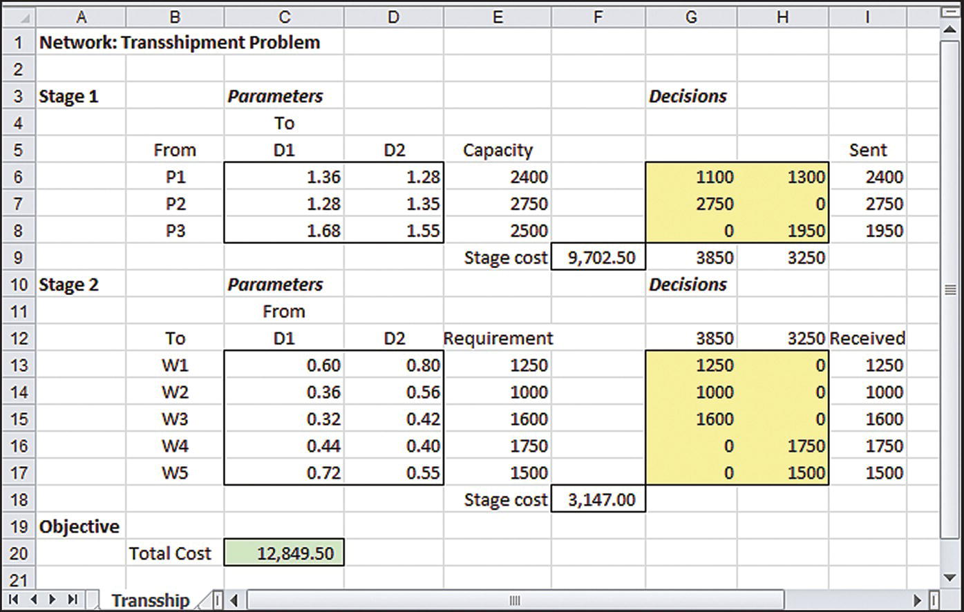
Figure 3.8 Spreadsheet model for Example 3.3.
In the upper portion of the model, the sources are represented in rows and the destinations are represented in columns. In the lower portion, this convention is reversed: The sources are represented in columns, and the destinations are represented in rows. Under this “flip-flopping” convention, the same columns (in this worksheet, columns C and D for costs or columns G and H for decisions) correspond to the DCs in both portions of the model. The identification of DCs with unique columns helps to reinforce the need for coordinating the flows into and out of the DCs. This structure also makes it relatively easy to accommodate an additional DC in the model (by inserting a column in the spreadsheet).
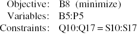
The model specification is as follows:

The formulation contains three LT constraints (one per plant), five GT constraints (one per warehouse), and two EQ constraints (one per DC). The optimal solution in this example is shown in Figure 3.8 with a total cost of $12,849.50. Thus, DeMont Chemical can take a systems view—and recognize both stages of its supply chain—when it optimizes its distribution costs.
To repeat, the total cost in cell C20 is the sum of the first-stage total cost and the second-stage total cost, and the decision variables appear in two arrays. Three types of constraints are needed in the model: a set of LT constraints for the plant capacities, a set of GT constraints for the warehouse requirements, and a set of EQ constraints balancing the inflows and outflows at the DC locations. Although this last set of constraints could also be expressed in the form of inequalities, the use of equations helps to identify the various constraints by associating a different constraint type (LT, GT, EQ) with each of the three different roles (capacities at the plants, requirements at the warehouses, and transshipment at the DCs). We can also view the EQ constraints as expressing the key conservation law of flows in networks: The total quantity flowing out of a node must always be equal to the total quantity flowing in.
To describe the conservation law algebraically, we introduce some notation for the decision variables. Let P2D1 represent the quantity shipped from plant P2 to DC D1, and so on. With this notation, we can write the conservation relationship for D1 as follows:

Similarly, for D2, we have
Thus, the conservation law takes the form of an equality constraint for particular nodes in the network. This equality constraint is sometimes called a balance equation, because it ensures perfect balance between inputs and outputs.
In this approach, we employed the conservation law to help build constraints for the DCs. We did not use the conservation law for the supply and demand nodes. At first glance, it may appear that the conservation law does not necessarily hold at those nodes. For example, if we interpret the input to node P1 as its capacity, we cannot be sure, before solving the optimization problem, whether all of that capacity will be used. Thus, we can’t tell whether the total flow out of the node will be equal to the flow into the node. A similar fact applies to the demand nodes, although as we noted earlier, we can expect the total flow into those nodes to equal the demands when there is an adequate supply in the network as a whole and when minimum cost is the objective. In other words, there is no economic incentive to violate the conservation law at the demand nodes, even though the constraints of the model might permit it. Nevertheless, there is a sense in which the conservation law holds even for the supply and demand nodes. We explore this interpretation in a later section.
3.4 FEATURES OF SPECIAL NETWORK MODELS
The transportation, assignment, and transshipment problems constitute a set of special network models in linear programming. They are special in the sense that they all lend themselves easily to the use of a flow diagram, and they all contain a from/to flow structure that leads directly to a row-and-column layout in a spreadsheet. In particular, we can conveniently display the decision variables as an array in the spreadsheet. When we specify the variables for Solver, we do not enter a row of adjacent cells, which is the standard format. Instead, we enter an array, or in the case of the transshipment model, a pair of arrays. (This feature could obviously be generalized to cases in which we have three or more stages in the model.) With the array format at the heart of the model, the constraints involve limitations on totals across a row or down a column. As a result, the constraints use the SUM formula, rather than the SUMPRODUCT formula that we saw throughout Chapter 2. Box 3.1 summarizes the prominent features of special networks.
One interesting feature of special network models is that an optimal solution always consists of an integer-valued set of decision variables whenever the constraint parameters are integer valued. Recall that the linearity assumption in linear programming allows for divisibility in the values of decision variables. As a result, some or all of the decision variables in an optimal solution may be fractional, and this sometimes makes the result difficult to implement or interpret. However, no such problem arises with special networks; they will always lead to integer-valued solutions as long as the constraint parameters are integers themselves.
Finally, the models of transportation, assignment, and transshipment problems introduced thus far have featured LT constraints for capacities and GT constraints for requirements, along with balance equations in the case of a transshipment model. In the case of the assignment model, its special structure allowed us to use equality constraints from the outset. However, as we shall discover next, it is possible to formulate any of these problems as linear programs built exclusively on balance equations. Although this approach may not seem as intuitive, it does link the flow diagram and the spreadsheet model more closely, as suggested at the beginning of the chapter.
3.5 BUILDING NETWORK MODELS WITH BALANCE EQUATIONS
The transportation model can easily be represented using the row-and-column format of the spreadsheet. However, we sometimes encounter other network structures that do not lend themselves quite as easily to an array layout. For these networks, it may be desirable to formulate the model using the standard linear programming format, with decision variables in a single row and with a SUMPRODUCT function in each of the constraints. In what follows, we provide a glimpse of how to approach network models in such a manner. The distinguishing feature of this approach is the use of balance equations, relying heavily on the information in a flow diagram. To illustrate how this approach works, we first return to examples we have already covered. As suggested earlier, the balance equation approach is not the most intuitive way to handle transportation, assignment, and transshipment problems, but it will be a useful background when we analyze other network models. By revisiting the transportation, assignment, and transshipment examples (Examples 3.1–3.3), we can explore a new approach while drawing on familiar problems.
The arcs of a network represent possible flow paths, and the quantities flowing along each arc correspond to decision variables in the model. For diagramming purposes, we also represent supply capacities and demand requirements as entering and leaving arcs, respectively, just as in Figure 3.1 or 3.5. Now, we take one additional step: We make sure that—for the entire network—the total supply quantity matches the total demand quantity. This feature allows us to write a balance equation for every node in the network.
Balanced totals for supply and demand occur in the assignment example of Figure 3.5. Since the problem comes to us with that feature, we can move from the diagram directly to the balance equations. For node A, the balance equation takes the following form:

Similarly, there are 11 other balance equations. The full spreadsheet model, with 36 variables and 12 constraints, is shown in Figure 3.9. The optimal solution produced by Solver achieves the minimum cost of $314 million, which we recognize from Figure 3.6. The set of assignments matches the optimal solution in the earlier formulation as well.

Figure 3.9 Standard linear programming format for Example 3.2.
It is not hard to imagine a problem in which total supply and demand are unequal. In fact, our transportation example in Figure 3.1 is just such a case. In this example, total supply is 40,000, while total demand is 39,000, so we have to deal with unbalanced totals for supply and demand. Here is how we proceed. We alter the diagram by adding a “dummy” warehouse to capture excess capacity. In our example, the requirement at this fictitious warehouse is 1,000, bringing demand and capacity into balance. We then add arcs linking each of the plants to the dummy warehouse, and we assign zero costs to these arcs.
We can think of shipments to the dummy warehouse as shipments to Nowhere. In other words, flows into the dummy warehouse are virtual flows that do not actually occur, whereas flows into the first four warehouses correspond to physical flows. The virtual flows correspond to unused capacity, which justifies using a cost of zero on these arcs. The complete diagram is shown in Figure 3.10. We see that the original diagram has been augmented so that there are now three capacities and five requirements, giving rise to 8 nodes, and there are 15 routes, corresponding to 15 arcs. However, the net effect has been to recast the original network into an equivalent one containing equal supply and demand quantities. This means that all of the supply available at the plants must ultimately find its way through the network to the warehouses. As a result, there must be a balance equation for every node.

Figure 3.10 Flow diagram for the augmented version of Example 3.1.
The next step is to translate the diagram into a linear programming model. We again set aside one variable for each arc; thus, we reserve 15 columns for decision variables. We also have eight constraints, one corresponding to each node. The essential requirement for any node in the model is a balance equation, that is, an EQ constraint ensuring that total flow into the node matches total flow out of the node, or
For example, at the Minneapolis node, the incoming flow corresponds to the capacity of 10,000, while the outgoing flows correspond to the arcs (decision variables) MA, MB, MC, MD, and MN. The balance equation becomes
or, in standard form, with variables on the LHS and constants on the right
For the other two plants, we obtain

For the Atlanta node, the incoming flow corresponds to the arcs MA, PA, and TA, while the outgoing flow corresponds to the requirement of 8000. The balance equation becomes
which we choose to write as
For the other destination nodes, we obtain

Figure 3.11 shows the complete spreadsheet model, in which all constraints are EQ constraints, and the objective function is unchanged from before. With the model in this form, we can distinguish flows into the network as positive RHS (in the first three constraints) from flows out of the network, which are negative RHS (in the last five constraints). The model specification is as follows:


Figure 3.11 Spreadsheet model for the augmented version of Example 3.1.
When we solve this optimization problem in the usual way, we obtain the same minimum cost we saw previously, $13,830, as shown in Figure 3.11. In this case, the decision variables also match those of Figure 3.2. The optimal solution also contains the decision variable TN = 1000, which we interpret as excess capacity of 1000 units at Tucson.
To summarize, we have followed a procedure for translating a network problem into a linear program. This procedure requires a flow diagram, possibly including a dummy node to capture unused capacity. Once we construct such a diagram, we can build the model by following these simple steps:
- Create a variable for each arc.
- Create a constraint for each node.
- Express each constraint as a balance equation.
In addition, a sign convention for RHS constants can provide improved clarity. Under this convention, a balance equation has a positive RHS to represent flow into the network and a negative RHS to represent flow out of the network.
For distribution problems of this sort, the from/to structure of the situation lends itself most readily to the special network layout shown in Figure 3.2, and that would be the modeling approach of choice. The approach suggested here is more general and would be valuable in situations that are more complicated than transportation, assignment, or transshipment problems. We examine some examples in the next section. Before we proceed, however, here is a perspective on the balance equation model.
The special network models all adhere to the conservation law and the use of balance equations, although it may be necessary to add a dummy node to make sure that all supply capacity is consumed. In the models we built at the outset, the addition of a dummy node and corresponding dummy arcs would have seemed unwieldy or unnecessary. Fortunately, we were able to avoid that step and proceed directly to a convenient formulation that contains inequalities rather than equations. In effect, we were dropping the dummy nodes and arcs from the network. By ignoring those virtual flows, we could change the balance equation for each supply node to an LT inequality. Similarly, we could also change the balance equation for each demand node to a GT inequality, incorporating the additional flexibility suggested in Chapter 2. These simplification steps left us with the network model we saw in Figure 3.2, but with our new perspective, we can interpret it as an adaptation of the balance equation model.
Special purpose solvers have been developed for use in industry and academia on large-scale network models. Typically, these procedures rely on balance equations and therefore require that formulations contain equality constraints. However, such procedures are not available in Solver. The use of balance equations with Solver may help avoid formulation errors, but it cannot exploit the algorithmic efficiencies that specialized network software packages offer.
3.6 GENERAL NETWORK MODELS WITH YIELDS
In network diagrams for the transportation, assignment, and transshipment models, arcs carry flow from one node to another. Moreover, on every arc, the flow into the destination node is implicitly required to exactly match the flow sent out from the source node. However, we can relax that kind of consistency requirement and extend network models to cases in which flows are subject to yield factors. The yield factors may shrink the amount flowing on an arc, in which cases we speak of a yield loss. Alternatively, yield factors may enhance the amount flowing, in which case we speak of a yield gain. The next two subsections provide examples of models containing yield factors.
3.6.1 Models with Yield Losses
Yield loss occurs in manufacturing processes where materials are shaped and trimmed to fit a target design, thus creating material waste. In other settings, quality inspections screen out defective parts. Process yields of these types reduce the amount of material in the main product. Similarly, yield loss may occur in distribution processes, especially with perishable goods: Fluids may partially evaporate during a delivery trip, or vegetables may spoil. The net effect of perishability, as with process yields, is simply a reduction in the amount of a flow that reaches its destination.
In this scenario, the yield factor tells us what proportion of the material sent along an arc will reach its destination. For the purposes of decision making, we can still measure the amounts sent out along each arc, but we have to adjust those figures to determine how much demand can actually be met at each destination. In addition, we cannot know in advance how much material in the aggregate will ship from the three plants. We know that, due to yield losses, we must ship more than the total demand quantity (still 39,000), but we can’t tell how much more because we don’t yet know which shipping routes we’ll use. Therefore, if we think of our model containing a demand node for nowhere, we must now treat the demand at that node as a variable.
For the purposes of illustration, we assume that each plant has a standard capacity of 16,000 units. Our supply constraints resemble those of the balance equation model in the previous section:
For the Atlanta node, the incoming flow corresponds to the net amounts on arcs MA, PA, and TA, while the outgoing flow corresponds to the requirement of 8000. The balance equation becomes
which we choose to write as
For the other destination nodes, we obtain

In this last constraint, NX measures the total quantity unshipped and does not appear in the objective function. The objective function is the same as the one we used initially.
Figure 3.12 shows the complete spreadsheet model, in which all constraints are EQ constraints, as in the previous section. In particular, the coefficients in rows 16–20 are yield factors, and these values are taken from the parameters in row 10. The model specification is as follows:


Figure 3.12 Spreadsheet model for Example 3.4.
When we solve this optimization problem in the usual way, we obtain the minimum cost of $15,498, as shown in Figure 3.12. To achieve this cost, the shipments out of Minneapolis and Pittsburgh exhaust capacity, whereas some excess capacity remains at Tucson. (The solution reflects this pattern because variables MN and PN are zero, but TN is positive.) From the model, we can determine that the total quantity shipped is 44,707, which provides the 39,000 units of demand after accounting for yields.
With yields present in the model, the structure is not as simple as the transportation model, but we can exploit the conservation law to help us develop valid constraints from balance equations.
3.6.2 Models with Yield Gains
We look next at flows that expand. Although there are chemicals that exhibit this property, a more familiar application involves money. As money flows through different locations in time, it usually expands. This expansion results from drawing interest or other kinds of investment returns. Consider the familiar problem of investing for college expenses.
Investment and funds-flow problems of this sort lend themselves to network modeling. In this type of problem, nodes represent points in time at which funds flow could occur. We can imagine tracking the balance in a bank account, with funds flowing in and out depending on our decisions. In Example 3.5, we include a node for now (time zero) and nodes for the end of years 1 through 7. Tracking time for this purpose, the end of year 3 and the start of year 4 are in effect the same point in time. To construct a typical start-of-year node, we first list the potential inflows and outflows that can occur.
- Inflows
- Initial investment
- Appreciation of investment A from 1 year ago
- Appreciation of investment B from 2 years ago
- Appreciation of investment C from 3 years ago
- Appreciation of investment D from 7 years ago
- Outflows
- Expense payment for the coming year
- Investment in A for the coming year
- Investment in B for the coming 2 years
- Investment in C for the coming 3 years
- Investment in D for the coming 7 years
Not all of these inflows and outflows apply at every point in time, but if we sketch the eight nodes and the flows that do apply, we come up with a diagram such as the one shown as Figure 3.13. In this diagram, A1 represents the amount allocated to Investment A at time zero, A2 represents the amount allocated to Investment A at the start of year 2, and so on. The initial investment in the account is shown as I0, and the expense payments are labeled with their numerical values. The diagram shows the different nodes as independent elements, which is all we really need; however, Figure 3.14 shows a tidier diagram in which the nodes are connected in a single-flow network.

Figure 3.13 Flow diagrams for Example 3.5.

Figure 3.14 Unified flow diagram for Example 3.5.
We do not need the variable B7 in the model. A 2-year investment starting in year 7 would extend beyond the 8-year horizon, so this option is omitted. However, the variable A8 does appear in the model. We can think of A8 as representing the final value in the account. Perhaps it is intuitive that if we are trying to minimize the initial investment, there is no reason to have money in the account at the end. Still, to confirm this intuition, we can include A8 in the model, anticipating that we will find A8 = 0 in the optimal solution.
The next step is to convert the diagram into a linear programming model. For this purpose, the flows in the diagram become decision variables. Then, each node gives rise to a balance equation, as listed below:

Figure 3.15 shows these EQ constraints as part of the spreadsheet model. A systematic pattern is formed by the coefficients in the columns of the constraint equations. Each column has two nonzero coefficients: a negative coefficient (of −1), corresponding to the time the investment is made, and a positive coefficient (reflecting the appreciation rate), corresponding to the time the investment matures. The only exceptions are I0 and A8, which essentially represent flows into and out of the network. In other funds-flow models, the column coefficients portray the investment-and-return profile on a per-unit basis for each of the variables. Following our sign convention, the RHS constants show the profile of flows in and out of the system over the various time periods. In this case, the constants in the last four constraints are positive, reflecting required outflows from the investment account in the last 4 years of the plan.

Figure 3.15 Spreadsheet model for Example 3.5.
The objective function in this example is simply the initial size of the investment account, represented by the variable I0, which we want to minimize. Thus, we can depart from the standard form (which normally uses a SUMPRODUCT function as the objective) and designate the objective function simply by referencing cell B5. The model specification is as follows:
When we minimize I0, Solver provides the optimal solution shown in Figure 3.15, calling for an initial investment of about $74,422. Compare this with the nominal value of the college expenses, which sum to $108,000. The lower figure for the initial investment testifies to the power of compound interest. In our example, the parents can use linear programming to take advantage of interest rate patterns and minimize the investment they need to make in order to cover the prospective costs of their daughter’s college education.
The nature of the optimal solution may not be too surprising. First, the return of 18% on the 3-year investment is dominated by the return of 6% on the 1-year investment A, due to compounding. Thus, we should not expect to see any use of the 3-year instruments in the optimal solution. The return on the 1-year investment is dominated, in turn, by the return on the 2-year investment and the return on the 7-year investment. Thus, we should expect to see substantial use of those two instruments. The use of the 1-year investment is dictated by timing: Because it is the only investment maturing at the end of year 5, it becomes the vehicle to meet the $26,000 requirement. Prior to that, the solution uses B3 (funded in turn by B1) to cover the first year of expenses and to fund A5. Then, B5 covers the third year of expenses, funded by B3. Finally, D1 covers the fourth year of expenses. As expected, the account should be empty at the end of the planning horizon.
The network diagram provides another perspective on this solution structure. In Figure 3.16, we show the network diagram, displaying only the positive flows. The diagram shows clearly that the only vehicle in the optimal solution for meeting the $30,000 requirement at node 7 is the investment in D1. Therefore, the size of the initial investment in D1 must be 30,000/1.65 = 18,182. Working backward, we can also see that the size of B5 is dictated by the $28,000 requirement and A5 is dictated by the $26,000 requirement. Once A5 and B5 are determined, they, together with the $24,000 requirement, dictate the size of B3. In turn, B3 dictates the size of B1. The diagram systematically conveys the detailed pattern in the optimal solution.

Figure 3.16 Flow diagram with optimal flows for Example 3.5.
Box 3.2 summarizes the important features of network models for funds-flow problems. In a multiperiod investment model, flows expand as they travel along arcs. Matter is not conserved as it flows, so we lose the conservation of matter that holds implicitly for flows between nodes in special networks. However, balance equations still apply at each node, in the sense that the total flow out of a node always equals the total incoming flow. The flows are still denominated in currency wherever they appear in the network. (Money is not converted into product, for example.) By contrast, we look next at a class of network models in which the flows are transformed.
3.7 GENERAL NETWORK MODELS WITH TRANSFORMED FLOWS
Another phenomenon that lends itself to network descriptions is the output of production processes. In this application, a node in the flow diagram represents a process that transforms inputs into outputs. In a transportation network, a node might represent a facility where material is received and ultimately sent out; however, the form of the input flow and the form of the output flow always match. That is, if the input is measured in truckloads, then so is the output. If the input is measured in cartons, then so is the output. The concept holds as well for nodes in a funds-flow network: If the input is measured in dollars, then so is the output. By contrast, production processes alter the material flowing in the system, so outputs may be made up of different material than the inputs from which they were created. Even with this generalization, network concepts are still applicable. Consider the example of oil refining at Delta Oil Company.

Figure 3.17 Flow diagram for Example 3.6.
We adapt the sketch of production flows and convert it to a standard network flow diagram by labeling each of the arcs in the network, recognizing that these labels can also serve as names of decision variables in a linear programming model. For convenience, we use some abbreviations, such as CR, which represents the amount of catalytic that is combined into regular gasoline. Next, we create node T to represent the tower and node C to represent the cracker. We also add nodes 1, 2, and 3 to represent allocations of flow. At node 1, the distillate must be split into a portion that is directly blended into gasoline and a portion that is used as a feedstock for the cracker. At node 2, the distillate allocated to blending must be split between regular and premium grades of gasoline, and similarly at node 3 for the catalytic produced by the cracker. Finally, nodes 4 and 5 represent the output of the two blending decisions, one for regular and one for premium.
For each node in the diagram, we write a balance equation. Conceptually, however, there is a twist here. Because the nodes represent transformation processes, the input material may differ from the output material, and there may be several input materials and output materials. (In distribution models and yield models, no transformation of material takes place.) We write a balance equation for each output material. For example, the equations for the tower node (T) take the following form:
Thus, this node generates two balance equations, one each for distillate and low-end by-products. Each equation contains one input term, for crude. The coefficients of 0.60 and 0.40 correspond to a fractional split of five barrels into flows of three barrels and two barrels, respectively, for the split between distillate (Dist) and low-end by-products (Low).
A similar pair of equations applies to the cracker node (C):

The numbered nodes are similar to transshipment nodes in our distribution models, because the inputs and outputs are the same material. At node 1, the distillate must be split into either feedstock (Feed) or gasoline blending input (Blend). The balance equation becomes
Nodes 2 and 3 have a similar structure:
Nodes 4 and 5 are also of this type:

The balance equations represent an algebraic description of the flow diagram. Conversely, the flow diagram represents a network representation of the balance equations. The system of balance equations and the network flow diagram are different manifestations of the same model. We can use one form to audit the other in order to check for consistency and eliminate structural errors.
The linear programming model has not been finished. In addition to the network “kernel” for this problem, other types of information are needed, including:
- Production capacities for each production process
- Sales potentials for final products
- Blending specifications for gasoline
The first two of these can be stated in appropriate dimensions, such as barrels per day, whereas the third describes limits on the ratio in which gasoline inputs may be mixed. To illustrate the entire model, suppose the following parametric assumptions apply:
- Tower and cracker capacities: 50,000 and 20,000 barrels/day
- Sales potential for regular and premium gasoline: 16,000 each
- Sales potential for by-products: unlimited
- Blending floor for catalytic in regular gasoline: at least 50% catalytic
- Blending floor for catalytic in premium gasoline: at least 75% catalytic
To complete the model, we need the economic factors that make up the objective function. Suppose the following parametric assumptions apply:
- Cost of crude oil: $28 per barrel
- Cost of operating the tower: $5 per barrel of crude
- Cost of operating the cracker: $6 per barrel of feedstock
- Revenue for high-end and low-end by-products: $44 and $36 per barrel
- Revenue for regular and premium gasoline: $50 and $55 per barrel
Figure 3.18 shows a spreadsheet model for the entire problem. Balance equations form the kernel of the model in rows 12–20. The next pair of constraints, in rows 21–22, contains the blending quality requirements for the grades of gasoline. Finally, the four constraints in rows 23–26 contain the ceilings on production capacities and sales volumes. These could alternatively be incorporated as upper bounds on the variables Crude, Feed, Reg, and Prem.

Figure 3.18 Spreadsheet model for Example 3.6.
The objective function is made up of revenue from the sales of outputs, the cost of operations, and the cost of input materials. For clarity, we devote a row of the spreadsheet to each of these components of the objective function, recognizing that several of these cells do not apply. In fact, intermediate products such as distillate are not directly associated with any costs or revenues at all. The value of the objective function, calculated as a SUMPRODUCT, appears in cell O9. The model specification is as follows:

Figure 3.18 displays the optimal solution to Delta Oil Company’s refining problem. In brief, the solution achieves a profit contribution of $466,400. It calls for purchases of 49,333 barrels of crude oil. This quantity leaves the tower with a small amount of excess capacity, but cracker capacity is fully utilized by the optimal allocation of distillate. Sales of regular gasoline are limited by market potential, but this is not the case for premium. Both gasoline products are blended at their minimum quality requirements, suggesting that catalytic is a scarce resource. A brief look at the decision variables reveals that there is flow on every arc in the network diagram.
Viewed as strategic information, the optimal solution provides useful insights into the determinants of profitability at Delta Oil. Of the two main pieces of process equipment, the cracker is currently the more constraining; however, the tower is not far behind. Capacity may have to be raised in both places for Delta to significantly increase its profits. On the output side, profits are also constrained by demand for regular gasoline. If the marketing department could find additional customers for regular gasoline, this could also lead to increased profits. In short, the strategic implications of the Delta Oil model are typical of product mix models; however, the construction of the model itself is driven by network-modeling principles.
Returning to the network structure, which lies at the heart of the Delta Oil model, we highlight the key features in Box 3.3.
SUMMARY
This chapter has introduced the network model to accompany allocation, covering, and blending models as one of the four basic linear programming types. The network model is uniquely adapted to the use of network flow diagrams, which can help substantially in constructing and debugging a spreadsheet model.
Among network models, a set of important cases is called special networks. Special network models arise frequently in distribution problems faced by industry. These models also have a structure that leads naturally to a distinctive array-based format for spreadsheet use. The use of arrays reflects the natural from/to structure in the problem itself, which lends itself readily to the row-and-column layout of a spreadsheet. (The array format adds an important case to the standard linear programming format covered in Chapter 2.) Special networks are usually formulated with inequality constraints; although from a more general perspective, these constraints are intuitive simplifications of a set of balance equations.
General network models illustrate the application of balance equations as a means of structuring an optimization problem. The overarching framework for these models is the same standard layout that was emphasized in Chapter 2. Nevertheless, the use of balance equations provides us with a simple recipe for developing a model (or a portion of a model) made up of EQ constraints. These constraints can be formulated directly from an accompanying flow diagram.
EXERCISES
- 3.1 Minimum Volume Requirements: Revisit the DeMont Chemical Company (Example 3.3). Notice that the flows in and out of the DCs are unconstrained, but suppose management wishes those volumes to be roughly similar. Add constraints to ensure that the volume at D1 and D2 will each be at least 40% of the total volume passing through the DCs.
- By how much does the optimal total cost increase as a result of these volume requirements?
- Which shipment quantities are altered by the imposition of the volume requirements?
- 3.2 Balance Requirements: Revisit the Goodwin Manufacturing Company (Example 3.4). Imagine a policy requiring that every shipping route must be used and, in particular, that the shipment volume on any route out of a plant must be at least 20% of the total volume leaving that plant.
- By how much does the optimal total cost increase as a result of the set of minimum requirements?
- How many shipment quantities are altered by the imposition of the “20% floor” requirements?
- 3.3 Stocking Warehouses: The Nicklaus Razor Blade Company plans to test market a new blade next month. The blades will be stocked in their three warehouses in the following quantities.
Warehouse A B C Stock (cartons) 50 50 50 Meanwhile, the carton quantities required by the distributors in the four test markets are as follows.
Distributor D E F G Requirement 45 15 25 20 The unit costs (in dollars per carton) of shipping the blades from warehouses to distributors are given in the table below.
D E F G A 8 10 6 3 B 9 15 8 6 C 5 12 5 7 - NRBC wishes to meet the distributor’s requirements at the minimum total transportation cost. Find the optimal plan.
- Show the network diagram corresponding to the solution in (a). That is, label each of the arcs in the solution and verify that the flows are consistent with the given information.
- 3.4 Distributing a Product: The Lincoln Lock Company manufactures a commercial security lock at plants in Atlanta, Louisville, Detroit, and Phoenix. The unit cost of production at each plant is 35.50, 37.50, 37.25, and $36.25, and the annual capacities are 18,000, 15,000, 25,000, and 20,000, respectively. The locks are sold through wholesale distributors in seven locations around the country. The unit shipping cost for each plant–distributor combination is shown in the following table, along with the forecasted demand from each distributor for the coming year.
Tacoma San Diego Dallas Denver St. Louis Tampa Baltimore Atlanta 2.50 2.75 1.75 2.00 2.10 1.80 1.65 Louisville 1.85 1.90 1.50 1.60 1.00 1.90 1.85 Detroit 2.30 2.25 1.85 1.25 1.50 2.25 2.00 Phoenix 1.90 0.90 1.60 1.75 2.00 2.50 2.65 Demand 5500 11,500 10,500 9,600 15,400 12,500 6600 - Determine the least costly way of shipping locks from plants to distributors.
- Show the network diagram corresponding to the solution in (a). That is, label each of the arcs in the solution and verify that the flows are consistent with the given information.
- Suppose that the unit cost at each plant were $10 higher than the original figure. What change in the optimal distribution plan would result? What if the plant costs were $20 higher?
- 3.5 Repositioning Supply: The American Rent-a-Car Company has eight outlets in a metropolitan area. American operates under a policy that calls for a specific “target” percentage of all available cars to be located at each outlet at the start of each day. These percentages are summarized in the following table.
Outlet 1 2 3 4 5 6 7 8 Percentage 20 10 20 5 10 20 5 10 For example, if 50 cars are available, 10 should be at outlet 1 at the start of the day. At the end of a day, if the current distribution of cars does not comply with the targets, American employees drive the cars overnight from outlet to outlet so that the new distribution meets the specified targets. The distance between each pair of outlets is given in the following table.
To Outlet 1 2 3 4 5 6 7 8 1 — 8 6 7 3 5 4 2 2 8 — 6 5 8 4 6 7 3 6 6 — 8 3 4 7 4 From Outlet 4 7 5 8 — 9 5 3 7 5 3 8 3 9 — 5 6 2 6 5 4 4 5 5 — 3 3 7 4 6 7 3 6 3 — 4 8 2 7 4 7 2 3 4 — At the end of a particular day, American finds that the 100 cars currently available are distributed at the outlets as follows.
Outlet 1 2 3 4 5 6 7 8 Cars 4 14 5 17 22 7 10 21 - Given this distribution of cars, find a schedule for minimizing the total distance traveled during the overnight redistribution of the cars.
- Show the network diagram corresponding to the solution in (a). That is, label each of the arcs in the solution and verify that the flows are consistent with the given information.
- 3.6 Assigning Tasks: A data processing department wishes to assign five programmers to five programming tasks (one programmer to each task). Management has estimated the total number of days each programmer would take if assigned to the different jobs, and these estimates are summarized in the following table.
Task 1 2 3 4 5 1 50 25 78 64 60 2 43 30 70 56 72 Programmer 3 60 28 80 66 68 4 54 29 75 60 70 5 45 32 70 62 75 - Determine the assignment that minimizes the total programmer days required to complete all five jobs.
- Show the network diagram corresponding to the solution in (a). That is, label each of the arcs in the solution and verify that the flows are consistent with the given information.
- How would the solution change if programmer 3 could not be assigned to tasks 2 or 4?
- 3.7 Distributing Oil: Texxon Oil Distributors, Inc., has three active oil wells in a west Texas oil field. Well 1 has a capacity of 93 thousand barrels per day (TBD), Well 2 can produce 88 TBD, and Well 3 can produce 95 TBD. The company has five refineries along the Gulf Coast, all of which have been operating at stable demand levels. In addition, three pump stations have been built to move the oil along the pipelines from the wells to the refineries. Oil can flow from any one of the wells to any of the pump stations and from any one of the pump stations to any of the refineries, and Texxon is looking for a minimum-cost schedule. The refineries’ requirements are as follows.
Refinery R1 R2 R3 R4 R5 Requirement (TBD) 30 57 48 91 48 The company’s cost accounting system recognizes charges by the segment of pipeline that is used. These daily costs are given in the tables below, in dollars per thousand barrels.
To Pump A Pump B Pump C Well 1 1.52 1.60 1.40 From Well 2 1.70 1.63 1.55 Well 3 1.45 1.57 1.30 To R1 R2 R3 R4 R5 Pump A 5.15 5.69 6.13 5.63 5.80 From Pump B 5.12 5.47 6.05 6.12 5.71 Pump C 5.32 6.16 6.25 6.17 5.87 - What is the minimum cost of providing oil to the refineries? Which wells are used to capacity in the optimal schedule?
- Show the network diagram corresponding to the solution in (a). That is, label each of the arcs in the solution and verify that the flows are consistent with the given information.
- 3.8 Cash Planning: A startup investment project needs money to cover its cash flow needs. The cash income and expenditures for the period January through April are as follows.
Month January February March April Total Cash flow ($000) −150 −450 500 250 150 At the beginning of May, all excess cash will be paid out to investors. There are two ways to finance the project. One is the possibility of taking out a long-term loan at the beginning of January. The interest on this loan is 1% per month, payable on the first of the month for the next 3 months. This loan can be as large as $400,000; the principal is due April 1; and no prepayment is permitted. The alternative is a short-term loan that can be taken out at the beginning of each month. This loan must be paid back at the beginning of the following month with 1.2% interest. A maximum of $300,000 may be used for this short-term loan in any month. In addition, investments may be made in a money market fund at the start of each month. This fund will pay 0.7% interest at the beginning of the following month. Assume the following about the timing of cash flows.
- For months in which there is a net cash deficit, sufficient funds must be on hand at the start of the month to cover the net outflow.
- For months in which there is a net cash surplus, the net inflow cannot be used until the end of the month (i.e., the start of the next month).
- What is the maximum amount that can be returned to investors? What is the optimal amount of money to borrow from each of the potential loan sources?
- Show the network diagram corresponding to the solution in (a). That is, label each of the arcs in the solution and verify that the flows are consistent with the given information.
- Explain the cost of funds for each month in the planning period. That is, if there were a $1000 change in the cash flows for any month, what would be the dollar change in the amount returned to investors?
- 3.9 Planning Cash: Each Fall, the treasurer of Trefny’s department store does financial planning for the next 6 months, September through February. Because of the holiday season, Trefny’s needs large amounts of cash during October, November, and December, whereas a large cash inflow is expected after the first of the year when customers pay off their holiday bills. The following table summarizes the predicted net cash flows (in thousands) from “business-as-usual” operations.
Month September October November December January February Surplus $20 — — — 30 150 Deficit — 30 60 90 — — The treasurer can draw on three sources of short-term funds to meet the store’s needs, although each represents a departure from “business as usual.” They are as follows:
- Accounts Receivable Loans. A local bank will loan Trefny’s funds on a month-by-month basis against a pledge on the accounts receivable balance as of the first day of a particular month. The maximum loan is 75% of the balance, and the cost of the loan is 1.5% per month, assessed on the amount borrowed. The predicted balances (in thousands) under “business-as-usual” plans are shown below.
Month September October November December January February Balance $70 50 70 110 100 50 - Delayed Payment of Purchases. All bills for purchases come due on the first of the month, but payments on all or part of these obligations can be delayed by 1 month. When payments are delayed this way, Trefny’s loses the 2% discount it normally receives for prompt payment under “business-as-usual” operations. (Loss of this 2% discount is effectively a financing cost.) The predicted payment schedule (in thousands) without the discount is shown below.
Month September October November December January February Payment $80 90 100 60 40 50 - Short-Term Loan. A bank is willing to loan Trefny’s any amount from $40,000 to $100,000 for 6 months, starting September 1. The principal would be paid back at the end of February, and Trefny’s would not be permitted to pay off part of the loan, or add to it, during the 6-month period. The cost of the loan is 1% per month, payable at the end of each month.
In any month, excess funds can be transferred to Trefny’s short-term investment portfolio, where the funds can earn 0.5% per month.
- Determine a plan for the treasurer that will meet the firm’s cash needs at minimum cost. (Assume that all cash flows occur at the beginning of the month.) What is the cost of this plan? Equivalently, what is the maximum amount of funds on hand after February?
- Show the network diagram corresponding to the solution in (a). That is, label each of the arcs in the solution and verify that the flows are consistent with the given information.
- Accounts Receivable Loans. A local bank will loan Trefny’s funds on a month-by-month basis against a pledge on the accounts receivable balance as of the first day of a particular month. The maximum loan is 75% of the balance, and the cost of the loan is 1.5% per month, assessed on the amount borrowed. The predicted balances (in thousands) under “business-as-usual” plans are shown below.
- 3.10 Planning a National Economy: The country of Utopia has a newly appointed Minister of International Trade. She has decided that Utopia’s welfare can be served best in the upcoming year by maximizing the net dollar value of Utopia’s exports (i.e., the dollar value of the exports minus the cost of the materials imported to produce the exports). The following information is relevant to this decision:
- Utopia produces only three products: steel, machinery, and trucks. For the coming year, the minister feels Utopia can sell all it can produce of these three products on the export market at the existing world market prices of 900 per ton of steel, 2500 per machine, and $3000 per truck.
- To produce one ton of steel, it takes 0.05 machines, 0.08 trucks, 0.5 person-years of labor, and imported materials costing $300. Utopia’s steel mills have the capacity to produce up to 300,000 tons/year.
- To produce one machine, it takes 0.75 tons of steel, 0.12 trucks, 5 person-years of labor, and imported materials costing $150. Utopia’s machinery plants have the capacity to produce up to 50,000 machines per year.
- To produce one truck, it takes 1 ton of steel, 0.1 machine, 3 person-years of labor, and imported materials costing $500. Utopia’s truck plants have the capacity to produce up to 550,000 trucks per year.
- The pool of labor in Utopia is equivalent to 1,200,000 person-years.
The minister plans to issue a self-sufficiency edict, declaring that Utopia cannot import steel, machinery, or trucks. She would like to determine the optimal production quantities and optimal export quantities for steel, machinery, and trucks when that edict is in force.
- Find the optimal export plan for Utopia’s economy, under self-sufficiency.
- Show the network diagram corresponding to the solution in (a). That is, label each of the arcs in the solution and verify that the flows are consistent with the given information.
- Describe, in simple terms that a nontechnical citizen can understand, the solution’s message to Utopia for how to manage its economy.