
1
Introduction to Prognostics
1.1 What Is Prognostics?
Prognostics is predictive diagnostics and provides the state of degraded health and makes an accurate prediction of when a resulting future failure in the system is likely to occur. The purpose of prognostics is to detect degradation and create predictive information such as estimates of state of health (SoH) and remaining useful life (RUL) for systems. Doing so yields the following benefits: (i) provides advance warning of failures; (ii) minimizes unscheduled maintenance; (iii) predicts the time to perform preventive replacement; (iv) increases maintenance cycles and operational readiness; (v) reduces system sustainment costs by decreasing inspection, inventory, and downtime costs; and (vi) increases reliability by improving the design and logistic support of existing systems (Pecht 2008; Kumar and Pecht 2010; O'Connor and Kleyner 2012).
Prognostics, as defined and used in this book, includes data acquisition (DA) and data manipulation (DM) by sensors (S) and processing within a sensor framework; DA, DM, and state detection (SD) employing processing and computational routines within a feature‐vector framework to produce feature data (FD) consisting of condition indicators that are leading indicators of failure (signatures); and health assessment (HA) and prognostic assessment (PA) within a prediction framework/prognostic‐information framework. The sensor framework, feature‐vector framework, prediction framework, and control and data flow framework form a prognosis subsystem within a prognostics and health management/monitoring (PHM) system (see Figure 1.1). Health management in a PHM system includes the generation of advisory information and health management/monitoring (HM): a health management framework (CAVE3 2015; IEEE 2017).
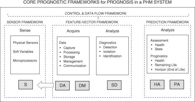
Figure 1.1 Core prognostic frameworks in a PHM system.
Source: based on IEEE ( 2017 ).
The focus of this book is prognostics although there is a strong linkage with System Health Management. Some aspects of health management are referenced and/or alluded to at times in the book. Included in this book is a framework for producing performance metrics to evaluate the accuracy of prognostic information. Figure 1.2 is a framework diagram for the exemplary PHM system used in this book.

Figure 1.2 Framework diagram for a PHM system.
Source: based on CAVE3 ( 2015 ).
1.1.1 Chapter Objectives
The scientific field encompassing the sensing, collecting, and processing of data to diagnose and provide a prognosis of the health of a system and estimates of future failure events is complex. Several prognostics concepts and solutions use a classical approach based on reliability theory and statistics: the fundamental ideas and methods of those classical approaches will be presented and discussed in this chapter. First, the basic ideas and methods of reliability engineering will be outlined, followed by brief discussions of the main ideas of the different elements of prognostic health management. This chapter includes some cost‐minimizing and cost‐benefit models.
The primary objective of this chapter is to provide a general overview of this complex scientific field. Detailed descriptions and model development for a heuristic approach to modeling condition‐based data (CBD) to support prognosis in a PHM system are presented in the later chapters.
1.1.2 Chapter Organization
The remainder of this chapter is organized to present and discuss a heuristic‐based approach to modeling CBD signatures as follows:
- 1.2 Foundation of Reliability Theory
This section presents the foundation upon which reliability is built: failure distributions, probability and reliability, probability density functions and relationships, failure rate, and expected value and variance.
- 1.3 Failure Distributions Under Extreme Stress Levels
This section presents models for failure and extreme stress, cumulative damage, and exponential and Weibull failures and distribution.
- 1.4 Uncertainty Measures in Parameter Estimation
This section presents an introduction to measurement metrics dealing with uncertainty, such as likelihood, variance, and covariance.
- 1.5 Expected Number of Failures
This section presents the effects and interaction of repair, replacement, and partial repair activities on assessing the number of failures and decrease in effective age due to partial repairs.
- 1.6 System Reliability and Prognosis and Health Management
This section presents a framework for a PHM system based on condition‐based maintenance (CBM) and introduces the reader to such a framework, CBD and signatures, and CBM, which can transform signatures into curves useful for processing to produce prognostic information.
- 1.7 Prognostic Information
This section introduces basic concepts and measures that are applicable to prognostic information: RUL, SoH, prognostic horizon (PH), prognostic distance (PD), and convergence.
- 1.8 Decisions on Cost and Benefits
This section presents a brief overview of decision problems and their mathematical modeling during different stages of the lifetime of equipment, with some illustrative mathematical models.
- 1.9 Introduction to PHM: Summary
This section summarizes the material presented in this chapter.
1.2 Foundation of Reliability Theory
Engineering systems and their components and elements are subject to degradation that sooner or later results in failure. A component that fails sooner compared to other components is said to be less reliable. Failures of like objects, such as components and assemblies, do not all occur at the same point in time; failures are distributed over time.
1.2.1 Time‐to‐Failure Distributions
The time to failure (TTF) of a particular object is usually modeled using probability theory, which represents the average behavior of a large set of identical objects and not the behavior of a particular object. It is considered as a random variable, denoted by X. The cumulative distribution function (CDF) of X is the probability that failure occurs at or before time t:
It is usually assumed that the object starts its operation at t = 0, so F(t) = 0 as t ≤ 0. Furthermore, F(t) tends to unity as t → ∞: the function is non‐decreasing. In reliability engineering, the most frequently used distribution types are as follows:
- Exponential distribution:1.2where the parameter λ > 0 determines the lifetime.

- Weibull distribution:
1.3where η > 0 is referred to as the scale and β > 0 is referred to as the shape.

- Gamma distribution:
1.4where k represents a shape parameter and θ represents a scale parameter. Furthermore, Γ(k) is the gamma function value at k. Very often, variable

 is used in applications.
 - Normal distribution:
1.5where μ is a real parameter and σ > 0.

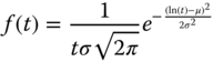
- Lognormal distribution:
1.6where μ is a real value and σ > 0. Here φ(t) is the standard normal distribution function defined in Eq. (1.7):
 1.7This does not have an exact simple formula; only function approximations are available, or the value of φ(t) for any particular value of t can be obtained from the corresponding function table.
- Logistic distribution:
1.8where μ and σ > 0 are the model parameters.

- Gumbel distribution:
1.9where the meanings of μ and σ are the same as before. This distribution is often called the log‐Weibull distribution.

- Log‐logistic distribution:
1.10where Eq. (1.10) also has an alternative formulation:
 1.11with α, β > 0 and α = eμ and
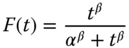

- Log‐Gumbel distribution:
1.12

- Log‐gamma distribution:
1.13where λ and α are positive parameters.

The CDFs of exponential and Weibull distributions are illustrated in Figures 1.3 and 1.4.
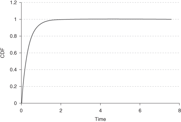
Figure 1.3 Graph of the exponential CDF with λ = 3.

Figure 1.4 Graph of the Weibull CDF with β = 1.2 and η = 5.
1.2.2 Probability and Reliability
Most probability values can be determined by using the CDF of X. The probability that failure occurs at or before time t is given as F(t), and the probability that the object is still working at time t is the complement of F(t),
which is called the reliability function of X. Sometimes it is also denoted by ![]() . The probability that failure occurs during time interval (t1, t2] is given as
. The probability that failure occurs during time interval (t1, t2] is given as
1.2.3 Probability Density Function
The probability density function (PDF) of X is the derivative of F(t):
- Exponential PDF:
It is easy to see that in the exponential case
1.17
- Weibull PDF:
1.18

- Gamma PDF:
The gamma PDF is the integrand of Eq. (1.4):
1.19
- Normal PDF:
The normal PDF has a closed form representation:
1.20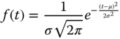
- Lognormal PDF:
1.21
- Logistic PDF:
1.22

- Gumbel PDF:
1.23

- Log‐logistic PDF:
1.24

- Log‐Gumbel PDF:
1.25

- Log‐gamma PDF:
1.26

The PDFs of exponential, gamma, and Weibull distributions are plotted in Figures 1.5–1.7.

Figure 1.5 Graph of the exponential PDF with λ = 3.


Figure 1.7 Graphs of Weibull PDFs.
Similar to the CDF of any random variable, most probability values can be obtained by using the corresponding PDF:


and

1.2.4 Relationships of Distributions
There is a strong relation between normal and lognormal, logistic and log‐logistic, gamma and log‐gamma, and Gumbel and log‐Gumbel distributions. If X is normal, then eX is lognormal; if X is logistic, then eX is log‐logistic; if X is Gumbel, then eX is log‐Gumbel and if X is gamma than eX is log‐gamma.
The domain of exponential, Weibull, gamma, and lognormal distribution functions is the [0, ∞} interval: that is, they are defined for positive arguments. However, in the normal case, t can be any real value. If the value of X can only be positive and we still want to use a normal distribution, then Eq. (1.20) must be modified:

where

And, therefore, the corresponding CDF is the following:

An exponential variable is very seldom used in reliability analysis since it doesn't model degradation or the aging of an object. In order to show this disadvantage, consider an object of age T, and find the probability that it will work for an additional t units of time. It is a conditional probability:

showing that this probability does not depend on the age T of the object. That is, the survival probability remains the same regardless of the age of the object.
Other important relations between different distribution types can be summarized as follows. If β = 1 in a Weibull variable, then it becomes exponential with ![]() . Assume next that X1, X2, …, Xk are independent exponential variables with an identical parameter λ; then their sum X1 + X2 + … + Xk is a gamma variable with parameters k and
. Assume next that X1, X2, …, Xk are independent exponential variables with an identical parameter λ; then their sum X1 + X2 + … + Xk is a gamma variable with parameters k and ![]() . Similarly, if X is exponential with parameter λ, then Xα is Weibull with parameters
. Similarly, if X is exponential with parameter λ, then Xα is Weibull with parameters ![]() and
and ![]() . Normal variables are characterized based on the central limit theorem, which asserts the following: Let X1, X2, …, XN, … be a sequence of independent, identically distributed random variables; then their partial sum
. Normal variables are characterized based on the central limit theorem, which asserts the following: Let X1, X2, …, XN, … be a sequence of independent, identically distributed random variables; then their partial sum ![]() converges to a normal distribution as N → ∞.
converges to a normal distribution as N → ∞.
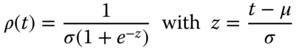
1.2.5 Failure Rate
The failure rate (or hazard rate) is defined mathematically as follows:
The numerator is the probability that the object will break down in the next Δt time periods given that it is working at time t. If Δt = 1, then the fraction gives the probability that the object will break down during the next unit time interval. By simple calculation,

which converges to the following:

That is, ρ(t) can be easily computed based on the PDF and reliability function of X. TTF distributions are characterized by their PDFs (f(t)), CDFs (F(t)), reliability functions (R(t)), and failure rates (ρ(t)). If any of these functions is known, then the other three can be easily determined as shown next.
If f(t) is known, then ![]() , R(t) = 1 − F(t), and
, R(t) = 1 − F(t), and ![]() .
.
If F(t) is known, then f(t) = F′(t), R(t) = 1 − F(t), and ![]() .
.
Assume next that R(t) is known. Then F(t) = 1 − R(t), f(t) = F′(t), and ![]() .
.
And finally, assume that ρ(t) is given. From its definition

and by integration

so

implying that
Exponential Failure
In the exponential case,
which is a constant and does not depend on the age of the object. This relation also shows that the exponential variable does not include degradation.
Weibull Failure
In the Weibull case,

which has different shapes depending on the value of β, as shown in Figure 1.8.
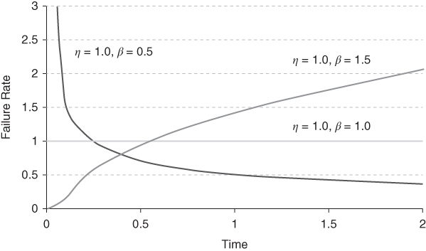
Figure 1.8 Failure rates of Weibull variables.
If β < 1, then the exponent of t is negative, so ρ(t) strictly decreases from the infinite limit at t = 0 to the zero limit at t = ∞. If β = 1, then ρ(t) is constant; and if 1 < β < 2, then the exponent of t is positive and below unity, so ρ(t) strictly increases and is concave in t. In the case of β = 2, the exponent of t equals 1, so ρ(t) is a linear function; and finally, as β > 2, the exponent of t is greater than 1, so ρ(t) strictly increases and is convex.
Gamma Failure
If X is gamma, then:
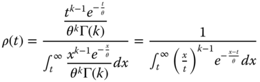
And by introducing the new integration variable u = x − t, we have:

If k = 1, then this is a constant since

and so ![]() . If <1 , then ρ(t) decreases; and if k > 1, then ρ(t) increases in t. Figure 1.9 shows the possible shapes of ρ(t), which always converge to
. If <1 , then ρ(t) decreases; and if k > 1, then ρ(t) increases in t. Figure 1.9 shows the possible shapes of ρ(t), which always converge to ![]() as t → ∞.
as t → ∞.

Figure 1.9 Failure rates of gamma variables.
Standard‐Normal Failure
Assume next that X is standard normal:

It is easy to show that ρn(t) strictly increases and is convex in t, ![]() ,
, ![]() , and
, and ![]() . Furthermore, the 45° line is its asymptote as t → ∞. The shape of ρn(t) is shown in Figure 1.10.
. Furthermore, the 45° line is its asymptote as t → ∞. The shape of ρn(t) is shown in Figure 1.10.

Figure 1.10 Failure rate of the standard normal variable.
Normal Failure
If X is a normal variable with parameters μ and σ, then ![]() ,
, ![]() , and
, and ![]() . Furthermore, its asymptote is
. Furthermore, its asymptote is ![]() as t → ∞.
as t → ∞.
Lognormal Failure
The failure rate of a lognormal variable X is shown in Figure 1.11. It is a mound‐shaped curve with a maximum at t*, which can be determined as follows. There is a unique value ![]() such that
such that ![]() , and then t*
, and then t* ![]() . Clearly
. Clearly
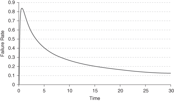
Figure 1.11 Failure rate of the lognormal variable with μ = 0 and σ = 1.
Logistic Failure
The failure rate of the logistic variable is
Gumbel Failure
In the case of the Gumbel distribution,
which is a simple exponential function.
Log‐Logistic Failure
Similarly, in the case of a log‐logistic variable:

Log‐Gumbel Failure
For the log‐Gumbel distribution,
as before.
Log‐Gamma Failure
The failure rate of the log‐gamma variable is

Figures 1.12–1.14 show the graphs of some of these failure rates.

Figure 1.12 Logistic failure rate with μ = 0 and σ = 1.


Figure 1.14 Log‐logistic failure rate with μ = 0.
1.2.6 Expected Value and Variance
The expected value and variance of any continuous random variable X can be obtained as follows:

where f(x) is the PDF of X:

The expectations and variances of the most frequently used random variables are summarized in Table 1.1, where γ ≈ 0.57721566 is the Euler constant.
Table 1.1 Expectations and variances.
| Type of distributions | Parameters | Domain | E(X) | Var(X) |
| Exponential | λ | [0, ∞) | 1/λ | 1/λ2 |
| Weibull | β, η | [0, ∞) | ||
| Gamma | k, θ | [0, ∞) | kθ | kθ2 |
| Normal | μ, σ2 | (− ∞ , ∞) | μ | σ2 |
| Lognormal | μ, σ2 | [0, ∞) | ||
| Logistic | μ, σ | (− ∞ , ∞) | μ | σ2π2/3 |
| Gumbel | μ, σ | (− ∞ , ∞) | μ − σγ | π2σ |
| Log‐logistic | μ, σ | (0, ∞) | eμΓ(1 + σ)Γ(1 − σ) | e2μ[Γ(1 + 2σ)Γ(1 − 2σ) − (Γ(1 + σ)Γ(1 − σ))2] |
The material of this section can be found in most introductory books on probability and statistics, as well as those on reliability engineering. See, for example, Ayyub and McCuen (2003), Ross (1987, 2000), Milton and Arnold (2003), Elsayed (2012), Finkelstein (2008), or Nakagawa (2008).
1.3 Failure Distributions Under Extreme Stress Levels
Traditional life data analysis assumes normal stress levels and other normal conditions. During operations, extreme stress levels may occur that significantly alter life characteristics. In this section, some of the most frequently used models are outlined. They play significant roles in reliability engineering, especially in designing accelerated testing.
1.3.1 Basic Models
We first discuss some of the most popular models.
Arrhenius Model
The Arrhenius life stress model (Arrhenius 1889) is based on the relationship
where L is a quantifiable life measure such as median life, mean life, and so on; V represents the stress level, formulated in temperature given in absolute units as Kelvin degrees; and B and C are model parameters determined by using sample elements.
This model is used mainly if the stress is thermal (i.e. temperature). We will next show how this rule is applied in cases of exponential and Weibull TTF distributions. Other distribution types can be treated similarly. Notice that L(V) is decreasing in V, meaning higher stress level results in shorter useful life.
The exponential PDF is known to be
where m is referred to as the expected TTF. Combining this form with Eq. (1.47) leads to a modified form of the PDF, which depends on time as well as on the stress level:

It can be shown that the expectation is ![]() , the median is
, the median is ![]() , the mode is zero, and the standard deviation is
, the mode is zero, and the standard deviation is ![]() . The Arrhenius‐exponential reliability function is
. The Arrhenius‐exponential reliability function is ![]() .
.
The Weibull PDF has the following form:

where the scale parameter is η. And the Arrhenius‐Weibull PDF can be derived by setting η = L(V), which gives the form

The expected value is ![]() , the median is
, the median is ![]() , the mode is
, the mode is  , and the standard deviation is
  .
.
Eyring Model
The Eyring formula (Eyring 1935) is used mainly for thermal stress, but it is also often used for other types of stresses. It is given as
where L, V, A and B have the same meanings as before.
In comparing the Eyring formula with the Arrhenius model, notice the appearance of a hyperbolic factor ![]() in the Eyring formula, which decreases faster in V than the Arrhenius rule.
in the Eyring formula, which decreases faster in V than the Arrhenius rule.
The Eyring‐exponential PDF can be written as follows:
since we chose m = L(V) as before. The mean is ![]() , the median is
, the median is ![]() , the mode is zero, and the standard deviation is
, the mode is zero, and the standard deviation is ![]() .
.
The Eyring‐Weibull PDF has a much more complicated form:

where we again selected η = L(V). It can be shown that the mean is ![]() , the median is
, the median is ![]() , and the mode is
, and the mode is  , with standard deviation

Generalized Eyring Model
The generalized Eyring relationship (Nelson 1980) is given by the more complex formula
where V is the thermal stress (in absolute units); U is the non‐thermal stress (i.e. voltage, vibration, and so on); and A, B, C, and D are model parameters.
In the case of a negative A value and C = D = 0, model Eq. (1.52) reduces to Eq. (1.50). Similar to previous cases, the modified generalized Eyring‐exponential PDF can be written as
where L(V, U) is given in Eq. ( 1.52 ). The mean is L(V, U), the median is L(U, V)·0.693, the mode is zero, and the standard deviation is again L(V, U).
The generalized Eyring‐Weibull PDF can be written as

with mean ![]() , median
, median ![]() , mode
, mode  , and standard deviation
Inverse Power Law
The inverse power law (Kececioglu and Jacks 1984) is commonly used for non‐thermal stresses:
where V represents the stress level, K and n are model parameters to be determined based on sample elements, and L is the quantifiable life measure. The power‐exponential and power‐Weibull probability density functions are given by Eqs. (1.53) and (1.54), where L(V, U) is replaced by Eq. (1.55).
Temperature‐Humidity Model
The most frequently used temperature‐humidity relationship is given as
The temperature‐humidity exponential and Weibull density functions are given by Eqs. ( 1.53 ) and ( 1.54 ), respectively.
Temperature‐Only Model
The temperature‐only relationship is based on the equation

which is a combination of the Arrhenius and inverse power laws. The corresponding exponential and Weibull PDFs are obtained again from Eqs. ( 1.53 ) and ( 1.54 ). Here, U is the non‐thermal stress (e.g. voltage, vibration, etc.), V is the temperature (in absolute units), and n and β are model parameters.
General Log‐Linear Model
In the case of multiple stresses, the function L(V) is usually substituted with a general log‐linear function:
where V1, V2, …, Vn are the different stress components, V = (V1, V2, …, Vn) is an n‐element vector, and a0, a1, …, an are model variables. The corresponding PDFs are obtained as before.
Time‐Varying Stress Model
Time‐varying stress models use different L(V) functions in the different sections of a time interval:
where t0 = 0 < t1 < t2 < … < tN = T, with T being the endpoint of the time span being considered.
Therefore, the corresponding PDFs are time‐varying: in each subinterval (ti, ti + 1), the corresponding Li(V) function represents the life measure under consideration.
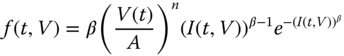
1.3.2 Cumulative Damage Models
Finally, we briefly discuss the cumulative damage relationship, where first the inverse power law is assumed. Let V(t) denote the time‐varying stress; then the life‐stress relationship is

where ![]() in comparison to Eq. ( 1.55
).
in comparison to Eq. ( 1.55
).
Exponential Failure Distribution
If the TTF distribution is exponential, then m(t, V) = L(V(t)). Defining

as the cumulative damage, the reliability function becomes e−I(t, V) and therefore the PDF has the form

Weibull Failure Distribution
If the TTF distribution is Weibull, then the reliability function is ![]() where I(t, V) is given by Eq. (1.61), and the corresponding PDF becomes
where I(t, V) is given by Eq. (1.61), and the corresponding PDF becomes
Exponential Failure Distribution and Arrhenius Life Stress
Assume next that the Arrhenius life stress model Eq. ( 1.47 ) is used. If the TTF is exponentially distributed, then similar to Eq. ( 1.61 ), we have

and the associated PDF becomes
Weibull Failure Distribution and Arrhenius Life Stress
If the TTF distribution is Weibull, then analogous to earlier cases η(t, V) = L(t, V), and therefore similar to Eq. (1.62) we get the associated PDF:
1.3.3 General Exponential Models
Next, we show the case of a general exponential relationship,
in which case

Failure Distributions
With exponential TTF distributions, the PDF becomes
And in the Weibull case,
If the general log‐linear function Eq. (1.58) is assumed, then

And in the exponential case, the corresponding PDF has the form
It is modified in the Weibull case as follows:

Reliability Function
The reliability function is
in the exponential or Weibull case. The CDF is clearly
The mean, median, mode, and variance can be obtained from the corresponding PDF or CDF by using standard methods known from probability theory.
Several books and articles have been written about accelerated testing, including Nelson (2004).
1.4 Uncertainty Measures in Parameter Estimation
Consider first a PDF that depends on only one parameter, θ, which is determined by using a finite sample. Let f(t|θ) denote the PDF, and let t1, t2, …, tN be the sample elements. The likelihood function is

and its logarithm is written as

which is then maximized to get the best estimate for the unknown parameter θ. By sampling repeatedly, we obtain different sample elements and therefore different estimates for θ. The value of θ depends on the random selection of the sample elements, so it is also a random variable. Its uncertainty can be characterized by its variance. Let the maximizer of Eq. (1.75) be denoted by θ*.
The Fisher information is defined as the negative of the second derivative of l(θ) with respect to θ at θ = θ*:

And it can be proved that the variance of θ is the reciprocal of I:
(Frieden 2004; Pratt et al. 1976).
If the distribution depends on more than one parameter – say, its PDF is f(t|θ1, …, θn) – then the likelihood function is

and its logarithm is

The Fisher information is now a matrix, the negative Hessian of l(θ1, …, θn):

It can be shown that the inverse matrix of I(θ1, …, θn) gives the covariance matrix of (θ1, …, θn).
1.5 Expected Number of Failures
The expected number of failures in a given time period [0, t] is an important characteristic of the reliable operation of an object, which may be an element, a unit, a block, or even an entire system. Clearly, this expectation depends on the way we react to failures. Three cases will be discussed in this section: minimal repair, partial repair, and failure replacement. We will also include lengths of time needed to perform repairs or replacements.
The material in this section is based on renewal theory, the fundamentals of which can be found, for example, in Cox (1970) and Ross (1996).
1.5.1 Minimal Repair
Consider first the case of minimal repairs, where each repair requires T time when the object is not operational. Let S1 denote the time of the first failure, M(t) the expected number of failures in the interval [0, t], and Xt the actual number of failures in this interval. Then
where

Therefore

where f(t) is the PDF of the TTF so that


In the special case when T = 0, this integral equation is modified as

where M(0) = 0. We will show that with the failure rate ρ(τ),
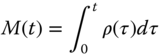
solves this equation by substitution. Notice first that based on the integration domain shown in Figure 1.15,


so the right side of Eq. (1.81) becomes

Figure 1.15 Integration domain.
The simple formula in Eq. (1.82) shows that {Xt} is a non‐homogenous Poisson process with arrival rate ρ(t), which has several important consequences. If the failures are independent, then Xt is a Poisson variable with λ = M(t) expectation, so
Assume that the repairable failures occur at times 0 < t1 < t2 < … and repairs are done instantly. Let Fk(t) denote the CDF of tk. Then

and the corresponding PDF is its derivative,


1.5.2 Failure Replacement
Assume next that upon failures, failure replacement is performed, which requires T time to complete. Then, similar to the previous case,

Therefore, Eq. (1.78) implies that


If t ≤ T, then the integral is zero, so

If replacement is instantaneous, then T = 0, so

gives the equation for M(t). There is no simple formula for the solution of this integral equation. However, the use of Laplace transforms provides an interesting insight. Let M*(s), F*(s), and f*(s) denote the Laplace transforms of M(t), F(t), and f(t), respectively. Then from Eq. (1.90), we have
implying that

If g(t) denotes the inverse Laplace transform of f*(s)/(1 − f*(s)), then

showing that {Xt} is again a non‐homogenous Poisson process with arrival rate g(t).
Let 0 < t1 < t2 < … denote times of failures. Then zk = tk + 1 − tk(k = 0, 1, … and t0 = 0) are independent random variables with PDF f(t). Then the density fk(t) of tk is the k‐fold convolution of f(t):
Notice that
where μ is the TTF mean value. Similarly
where σ2 is the TTF variance value. If zk is exponential, then tk is gamma; if zk is gamma, then tk is also gamma; and if zk is normal, then tk is also a normal variable.
Based on these values, in other cases the PDF of tk can be estimated by a lognormal or gamma variable with a given expectation and variance; and confidence intervals can be constructed for any significance level selected by the user.
If repairs or replacements need T time to perform, then the time of the kth failure is ![]() , with the CDF
, with the CDF

where Fk(t) is the CDF of fk(t).
1.5.3 Decreased Number of Failures Due to Partial Repairs
Assume next that partial repairs are performed, resulting in the number of failures decreasing by a factor of α < 1. Then, similar to the previous cases,

So


Assume again instantaneous repairs with T = 0. Then (1.94) is modified as

1.5.4 Decreased Age Due to Partial Repairs
Consider finally the case where partial repairs decrease the effective age of the object by a factor α < 1. Then we have

since at time t the effective age is (t − S1 − T) + αS1, where the first term is the length of interval [S1 + T, t] and the second term is the effective age at time S1 + T after repair. Therefore


If T = 0 then

Notice that the case α = 1 corresponds to minimal repair, and Eqs. (1.95) and (1.98) reduce to Eq. ( 1.81 ) as they should. Equations ( 1.81 ), ( 1.90 ), and ( 1.95 ) are usually called the renewal equations (Mitov and Omey 2014).
The value of M(t) for given values of t usually requires the solution of integral equations; however, in the case of model Eq. ( 1.81 ), the solution was given in a simple formula. Assume first that the cost of each repair is cr and no discounting of money is considered. The total repair cost in interval [0, t] is clearly crM(t) in the average.
Let r denote the discount factor, and assume minimal repair each time. Then the expected discounted cost in interval [0, t] is the following:


1.6 System Reliability and Prognosis and Health Management
A PHM system is complex and comprises several subsystems. In the classical approach, this complex system is based on probabilistic considerations that have many disadvantages in comparison to the new approach that will be introduced and discussed in this book. First, the probability distributions reflect the average behavior of many identical items, not the behavior of one particular item under consideration. Second, the parameters of the distribution functions used in the process are not exact; their parameters are uncertain, as demonstrated earlier. A more practical approach is to use CBD, from which you extract feature data (FD) consisting of leading indicators of failure; then, as necessary, perform signal conditioning, data transforms, and domain transforms to create data that forms a fault‐to‐failure progression (FFP) signature. FFP signatures have been successfully processed by prediction algorithms to produce accurate estimates of system health and remaining life. Increased accuracy is achieved by further transforming FFP signature data in degradation progression signature (DPS) data and then transforming DPS data into functional failure signature (FFS) data. FFS data processed by predication algorithms employing Kalman‐like filtering, random‐walk, and/or other trending algorithms results in very accurate prognostic estimates and rapid convergence from, for example, an initial error of 50% to 10% within fewer than 20 data samples. This rapid, accurate convergence is very useful for CBM in PHM systems (Hofmeister et al. 2016, 2017a,b).
1.6.1 General Framework for a CBM‐Based PHM System
Figure 1.16 illustrates a PHM system forming a framework for CBM. The system monitors, captures, and processes CBD to extract signatures indicative of the state of health (SoH) of devices, components, assemblies, and subsystems in systems. Extracted signatures are processed to produce prognostic information, such as SoH and RUL, which are further processed to manage maintenance and logistics of the system (CAVE3 2015 ; Hofmeister et al. 2016 ).

Figure 1.16 High‐level block diagram of a PHM system.
Figure 1.17 is an exemplary illustration of a framework for CBM. The framework consists of (i) a sensor framework, (ii) a feature‐vector framework, (iii) a prediction framework; (iv) a health‐management framework, (v) a performance‐validation framework, and (vi) a control‐ and data‐flow framework.

Figure 1.17 A framework for CBM for PHM.
Source: after CAVE3 ( 2015 ).
A sensor framework comprises sensors to capture signals at nodes within the system. Smart sensors provide initial data conditioning such as analog‐to‐digital data conversion and digital‐signal processing, and produce and transmit FD such as scalar values. A feature‐vector framework provides additional data conditioning, including data fusion and transformation to create signatures, such as FFS that are used as input data to a prediction framework that produces prognostic information. A health‐management framework processes prognostic information to create diagnostic, prognostic, and logistics directives and actions to maintain the health and reliability of the system. A performance‐validation framework provides means and methods to produce prognostic‐performance metrics for evaluation of the accuracy of prognostic information. A control‐ and data‐flow framework manages PHM functions and actions (CAVE3 2015 ; Pecht 2008 ; Kumar and Pecht 2010 ).
Reliability R(t) (refer back to Eq. (1.14) of a prognostic target is the probability that the prognostic target will operate satisfactorily for a required period of time. Reliability is related to lifetime and mean time before failure (MTBF) by the following (Speaks 2005). Theoretically, the mean time before failure is obtained from probabilistic reasoning as the expectation of TTF:

where f(t) is a PDF. By examining a number of test units, it can be obtained practically as
where N= number of test units, T= test time, and F= number of test failures.
The relative frequency of number the of failures until time T is clearly given as F/N, which is an estimator of the CDF of TTF at time t = T. If the distribution is exponential, then its parameter can be estimated from
so an estimate of λ is
Then the CDF is given as F(t) = 1 − e−λt, the reliability function is R(t) = e−λt, and the constant failure rate is λ. We previously derived these results; refer back to Eq. (1.2), for example. If the distribution of TTF has more than one parameter, then the information provided by λ is not sufficient to estimate R(t). For example, the variance can be estimated by repeated testing, so two equations would be obtained for the usual two parameters (such as Weibull, gamma, normal, and so on).
MTBF is a statistical measure that applies to a set of prognostic targets N and is not applicable for estimating the lifetime or RUL of a specific prognostic target in a system.
1.6.2 Relationship of PHM to System Reliability
What is the relationship of PHM to system reliability? As an example, suppose a PHM system is designed to accurately predict the time when functional failure will occur for every prognostic target in the system; further suppose that the fault/health management framework of that system enables replacement and/or repair of every prognostic target prior to the actual time of functional failure; also suppose that the time when maintenance is performed occurs after the time when degradation is detected for each prognostic target; and also suppose that the time to replace and/or repair prognostic targets in a PHM‐enabled system is less than the time to replace and/or repair unexpected outages. In such a PHM‐enabled system, the effective MTBF of the system is increased, and therefore the reliability of the system is also increased. In addition to increasing the reliability of the system, PHM reduces the cost of maintaining the system because the operating lives of the prognostic targets are increased and because it is generally less expensive, in both time and materials, to handle planned versus unexpected outages.
Any number of traditional modeling approaches lend themselves as base platforms for PHM‐enabling systems that can be classified as model‐based prognostics, data‐driven prognostics, or hybrid‐driven prognostics (see Figure 1.18). Model‐based approaches often offer potentially greater precision and accuracy in prognostic estimations, which can be difficult to apply in complex systems. Data‐driven approaches are simpler to apply but can produce less precision and less accuracy in prognostic estimations. Hybrid‐driven approaches offer a high degree of precision and accuracy and are applicable to complex systems, including on‐vehicle and off‐vehicle, taking advantage of both approaches (Pecht 2008 ; Medjaher and Zerhouni 2013).

Figure 1.18 Taxonomy of prognostic approaches.
In Chapter 2, we will return to these concepts and approaches in more detail.
1.6.3 Degradation Progression Signature (DPS) and Prognostics
A CBM system, such as that presented in this book, uses a CBD approach. As a prognostic target in a system progresses from a state of no damage (zero degradation) to a state of damage (degraded) and then to a failed state, one or more signals at one or more nodes in the system will change. Such signal changes can be sensed, measured, collected, and processed by a PHM system to produce highly accurate prognostic information for use in fault and/or health management. As an example, suppose a power supply in a system becomes damaged, and the ripple voltage of the output changes and increases as the amount of damage (accumulated degradation) in the power supply increases. Further, suppose the amplitude of the ripple voltage can be sensed, measured, and collected by a sensor framework in a PHM system. The collection of CBD amplitudes forms an FFP signature, such as that shown in Figure 1.19.

Figure 1.19 Example of an FFP signature – a curvilinear (convex), noisy characteristic curve.
Clearly the FFP curve is not smooth, due to the effects of measurement uncertainty and noise. Now suppose a feature‐vector framework in that PHM system consists of data‐conditioning algorithms that filter, smooth, fuse, and transform CBD‐based FFP signatures into DPS data: a transfer curve. An ideal DPS has a constant steady‐state value in the absence of degradation; it linearly increases in correlation to the level of degradation; and it reaches a maximum amplitude when the level of degradation is at its maximum: physical failure occurs. For this example, such an ideal DPS is shown as the line with positive slope in Figure 1.20; also shown are the points at which the onset of degradation occurs and when physical failure occurs.

Figure 1.20 Ideal DPS transfer curve superimposed on an FFP signature.
Further suppose a PHM system allows a reliability engineer to specify a noise margin to mask signal variations due to, for example, environmental and operational noise. An example of a noise margin is that indicated by the lower horizontal line on the plot in Figure 1.21. Also suppose a PHM system allows a reliability engineer to specify a level of degradation that defines a threshold at which a prognostic target is no longer capable of satisfactorily operating within specifications: functional failure occurs, as indicated by the circled Functional Failure point in the plot shown in Figure 1.21 . A PHM system can be designed to support reliability R(t) with emphasis on operating satisfactorily, meaning to operate within a required set of specifications: a functional‐failure threshold used for transforming a physical‐failure‐based DPS into an FFS, such as that shown in Figure 1.22.

Figure 1.21 Ideal DPS, degradation threshold, and functional failure.

Figure 1.22 Normalized and transformed FFP and DPS transformed into FFS.
1.6.4 Ideal Functional Failure Signature (FFS) and Prognostics
Now suppose the PHM system transforms FFS amplitudes into percent values, as shown in Figure 1.23. Transforming CBD into a DPS and then into an FFS creates useful input data for prediction algorithms to produce accurate prognostic information: (i) when FFS = 0, no degradation; (ii) when FSS > 0 and < 100, degradation but operating within specifications; and (iii) when FFS = 100, functional failure has occurred.

Figure 1.23 Ideal FFS – transfer curve for CBD.
To further illustrate the usefulness of FFS transfer curves, suppose a PHM‐enabled system has three similar prognostic targets for which ideal DPS transfer curves are shown in Figure 1.24. The plots exhibit four significant variabilities: (i) each prognostic target starts to degrade at a different sample time; (ii) each prognostic target has a different nominal value in the absence of degradation; (iii) each prognostic target has a different rate of degradation; and (iv) each prognostic target exhibits a different amplitude at physical failure. Included in the plots are the horizontal lines representing the thresholds specified by a reliability engineer for noise (below) and functional failure (above).

Figure 1.24 Variability in DPS transfer curves.
Now suppose the PHM system and its prediction algorithms are designed to translate clock time to relative time with respect to the detection of degradation during prognostic processing; and also suppose the PHM system and its prediction algorithms truncate FFS values to 0 and 100. Then the plots of the FFS transforms are shown in Figure 1.25.

Figure 1.25 FFS transforms of the DPS plots shown in Figure 1.23 .
The design of a prediction algorithm to produce accurate prognostic information is greatly facilitated when FFS data is the input. For example, at any relative sample time (ST), the corresponding sample amplitude (SA) is used to calculate an estimated failure time (FT), RUL, and SoH using the following equations:
1.6.5 Non‐ideal FFS and Prognostics
In practice, it generally is not possible to obtain ideal FFS transfer curves. Instead, the curves will be noisy and distorted, and will exhibit changes associated with changes in the degradation rate – similar to what is shown in Figure 1.27. Small perturbations may be due to measurement uncertainty and have no relationship or significance with respect to the actual SoH and/or RUL of a prognostic object: in such cases, prediction algorithms should employ methods to filter or otherwise mitigate these variations. On the other hand, an FFS change might be caused by a real, significant change in the rate of accumulated damage in a prognostic target: in such cases, prediction algorithms should employ methods to recognize and take into account these changes in degradation rates, which should modify the estimates of SoH and RUL. Mitigation of and accounting for both causes of signal variability are competing objectives in the design of prediction algorithms: in practice, to design of prediction algorithms that satisfy both objectives, the algorithms need to incorporate appropriate design compromises. In subsequent chapters of this book, you will see examples of how FFS variabilities are successfully handled.

Figure 1.27 FFS transfer curve exhibiting distortion, noise, and change in degradation rate.
1.7 Prognostic Information
Prognostic information includes the following significant metrics: RUL, SoH, and PH. Figure 1.28 shows example plots of an ideal RUL and ideal PH: (i) the estimated time of failure relative to the onset of degradation is PH, and the initial value specified by a reliability engineer is exactly correct; (ii) the onset of degradation is detected exactly at the time the prognostic target begins to degrade; (iii) the time when degradation reaches the specified level for failure is exactly detected; and (iv) the FFS input to a prediction algorithm is ideal. The PH and RUL plots are perfectly linear, with no noise or distortion – the RUL is an exact linear progression from 200 to 0 days.

Figure 1.28 Example plots of an ideal RUL and ideal PH.
Similarly, Figure 1.29 shows the plots of an ideal SoH and an ideal PH accuracy. SoH is an exact linear progression from 100% to 0%, and PH accuracy is exactly 100% before and after the onset of degradation.

Figure 1.29 Example plots of an ideal SoH transfer curve and PH accuracy.
1.7.1 Non‐ideality: Initial‐Estimate Error and Remaining Useful Life (RUL)
A major cause of non‐ideality in prognostic information is the difference between an estimated TTF of a prognostic target defined by a reliability engineer (an initial RUL estimate) and the actual TTF between the onset of degradation and functional failure. It is extremely unlikely that estimated initial TTF values will exactly equal actual TTF values, and therefore there will be initial‐estimate errors. For example, in Figures 1.28 and 1.29 , the defined TTF value is 200 days and is exactly equal to the true TTF value at functional failure. But suppose a reliability engineer had estimated the TTF after the onset of degradation to be 300 days. In that case, when degradation is detected, the estimated RUL will be 300 days, and the actual TTF will be 200 days – an initial error of 100 days, as shown in Figure 1.30.
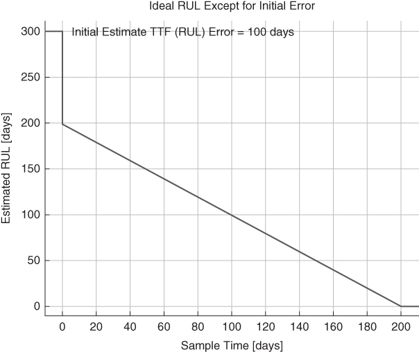
Figure 1.30 Example of RUL with an initial‐estimate error of 100 days.
1.7.2 Convergence of RUL Estimates Given an Initial Estimate Error
It is desirable to design prediction algorithms that (i) mitigate FFS variability not caused by degradation and (ii) respond to FFS variability caused by degradation. A design approach is to treat FFS data points as particles having inertia and momentum. Particles do not exhibit rapid changes; instead, they tend to maintain velocity and direction. A satisfactory design objective is to employ a dampening factor for changes in amplitude and velocity. Another design approach is to develop a random‐walk solution for particles that progress from a zero‐degradation state (lower‐left corner) to a maximum‐degradation state (upper‐right corner) – a solution that employs Kalman‐like filtering (Hamilton 1994; Bucy and Joseph 2005): (i) use the previous data point of an FFS model; (ii) calculate the predicted location of the next data point; (iii) adapt the FFS model to an adjusted location between the predicted and the actual location of the next data point; (iv) use dampening factors and coefficients to adjust the FFS model; (v) use the adapted FFS model to estimate when functional failure is likely to occur; and (vi) calculate prognostic information such as RUL, SoH, and PH.
1.7.3 Prognostic Distance (PD) and Convergence
Referring back to Figures 1.31 and 1.32 , the dotted horizontal lines represent a desired zone of accuracy called alpha (α). A prognostic parameter of interest is the prognostic distance when prognostic estimates RUL and PH are within an application‐specific value α (Saxena et al. 2009):
1.7.4 Convergence: Figure of Merit (χα)
The convergence efficiency of a prediction algorithm is dependent on many factors, including the following:
- The dampening used in the design of the prediction algorithm. A large dampening factor increases the number of FFS data points required to converge to a desired level of accuracy.
- The value of the initial‐estimated TFF. The larger the initial error, the more FFS data points need to be processed to converge to a desired level of accuracy.
- The CBD rate of sampling. The slower the sampling rate, then even if the amount of data processed remains the same, the time between data points is increased, and the longer it takes to reach a desired level of accuracy.
Failure of a prediction algorithm to meet your requirements for convergence efficiency might be caused by many factors other than design, including (i) errors in specifications, such as the initial‐estimated value for TTF; (ii) design or operational specifications of the sensor framework; and (iii) insufficient data conditioning that results in overly detrimental offset errors, distortion, and noise in the FFS input.
1.7.5 Other Sources of Non‐ideality in FFS Data
Other sources of non‐ideality in FFS data include, but are not limited to, the following: (i) offset errors in detecting the onset of degradation and the time of functional failure; (ii) distortion in FFS data due to the effects of using noise margins; (iii) measurement uncertainty associated with, for example, quantization errors of data converters; (iv) unfiltered variability caused by environmental effects such as voltage and temperature; and (v) the effects of self‐healing as the operational and/or environment of a prognostic target changes. Figure 1.33 illustrates a non‐ideal FFS and the effects of some of the causes of the non‐ideality.

Figure 1.33 Example of FFS data exhibiting an offset error, distortion, and noise.
1.8 Decisions on Cost and Benefits
Over the lifetime of any equipment, hard decisions arise regarding the choice of the right or best equipment to purchase; selection, inspection, maintenance, and repair strategies; and finding the optimal time for preventive replacement in order to avoid costly failures that might result in additional damage or accidents. This section gives a brief overview of the decision problems and their mathematical modeling during different stages of the lifetime of equipment, with some illustrative mathematical models.
1.8.1 Product Selection
There are usually several alternative choices of similar equipment available for purchase, and the choice must be based on several criteria. This leads us to use multi‐objective optimization techniques. (Szidarovszky et al. 1986) give a summary of the different concepts and algorithms for solving such problems, so we will not give those details; instead, this section of the book will provide an illustrative example to provide an idea of their usage.
1.8.2 Optimal Maintenance Scheduling
The objective of any maintenance action is either to retain the condition of the object under consideration or to restore it to the desired condition. Therefore, we can divide maintenance actions into two major groups: preventive and corrective maintenance types.
If maintenance is carried out at predetermined time intervals without checking the condition of the item, we are referring to predetermined maintenance. If the item is regularly monitored, condition‐based maintenance can be performed. This can result in either improving the item without changing its required function; or in modifying it, if the required function of the item is altered. If failure is detected, then after the fault is diagnosed, it is corrected. And finally, the operation of the item is checked out to be sure the repair was done correctly and successfully.
In this section, some mathematical models for optimal maintenance scheduling will be introduced.
Predetermined Maintenance
First, we introduce a model for scheduling predetermined maintenance actions. Consider a piece of equipment that is subject to preventive maintenance actions, which are performed in a uniform time grid. Between maintenance actions, only minimal repairs are performed, in cases of failure. Let h denote the length of time between consecutive maintenance actions. Without maintenance, let F(t), f(t), R(t), and ρ(t) denote the CDF, PDF, reliability function, and failure rate of time to non‐repairable failure.
In addition to the value of h, two other decision variables can be introduced. One characterizes the level of maintenance, so as a result of each maintenance action the effective age of the equipment decreases by u, where 0 < u < h. It must also be determined how long the equipment is scheduled to operate, which can be represented by a positive integer n showing that when the nth maintenance is due, the equipment is replaced. So, maintenance actions are performed at times h, 2h, …, (n − 1)h, and the equipment is replaced at time nh. For k = 1, 2, …, n, let Fk(t), fk(t), and ρk(t) denote the CDF, PDF, and failure rate of the equipment in interval [(k − 1)h, kh]. Then clearly
Before the model of cost minimization is developed, an important constraint must be presented. The reliability of the equipment must not go below a user‐selected threshold r0:
implying that
For example, in the case of a Weibull distribution, Eq. (1.108) can be written as
By taking the logarithm on both sides we get

or
which is a linear constraint.
The expected net cost per unit time is minimized. The following factors must be considered:
- The cost of preventive replacement is cp, whereas the cost of failure replacement is cf > cp.
- Repairable failures may occur with failure rate
 . Then, assuming minimal repair, the expected number of such failures in any interval (t1, t2) is given as
  . Each repair costs cr.
 - The cost of each maintenance action depends on the level of maintenance: a + bu by assuming the linear constraint of Eq. (1.110).
- The revenue‐generating density of the working equipment is assumed to be A − BT, where T is the effective age of the equipment. So, revenue generated between effective ages T1 and T2 is the integral
1.111

- After the equipment is replaced at time t, it is assumed that its salvage value is Ve−wt, where V is the value of a new piece of equipment, and as time progresses the value of the equipment decreases exponentially.
In computing the expected cost per unit time, we have to consider two cases:
- Case 1. The equipment does not face non‐repairable failure before the scheduled replacement time. Then the net cost per unit of time is given as
1.112

The first term is the cost of preventive replacement, the second term is the overall cost of maintenance actions, and the third term is the cost of repairs. The last two terms represent the salvage value and the generated revenue.
The last term can be further simplified:

Let's denote Eq. (1.112) as COST1 (n, h, u).
- Case 2. Non‐repairable failure occurs at a time t ∈ ((k − 1)h, kh]. Then the net cost per unit time is


 1.114
1.114
where we used Eq. (1.113) with k − 1 instead of n and Eq. (1.111) for the interval
Notice that in computing the repair costs and generated revenue, in addition to the intervals (0, h], (h, 2h], …, ((k − 2)h, (k − 1)h], we have to take into account the last interval ((k − 1)h, t] as well. Equation (1.114) can be denoted by COST2(t, k, h, u).
Then the expected net cost per unit time during a complete cycle (until replacement) is given as

which is minimized with respect to decision variables 0 < u < h, n ∈ {1, 2, …}. We have to assume that the revenue generating density is positive: A − Bnh ≧ 0; otherwise the machine would produce loss.
The previous formulation considered one type of repairable and non‐repairable failures. If I types of repairable failures are considered, the third terms of Eqs. ( 1.112
) and ( 1.114
) have a second summation with respect to i before cr, which is replaced by cri; and ![]() must be replaced by
must be replaced by ![]() . These represent the cost and number of repairable failures of type i. Assume next that there are J types of non‐repairable failures with CDFs F(j)(t) for j = 1, 2, …, J. Let the failure times be denoted by X(j), j = 1, 2, …, J. The first non‐repairable failure occurs at X = min {X(1), X(2), …, X(J)}, with CDF
. These represent the cost and number of repairable failures of type i. Assume next that there are J types of non‐repairable failures with CDFs F(j)(t) for j = 1, 2, …, J. Let the failure times be denoted by X(j), j = 1, 2, …, J. The first non‐repairable failure occurs at X = min {X(1), X(2), …, X(J)}, with CDF


by assuming that the non‐repairable failures are independent of each other.
Optimal Coordination
In the next related model, the optimal coordination of the maintenance actions of several machines will be discussed. Consider a machine shop with K machines with equal lifetime of N time periods. The maintenance of these machines must be scheduled optimally in order to reduce setup costs. Let
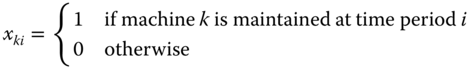
for i = 1, 2, …, N and k = 1, 2, …, K
The constraints are as follows:
- For machine k, the time difference between consecutive maintenance actions must not be more than mk: at least one maintenance must be done during the first mk time periods:
and in general
 1.116
1.116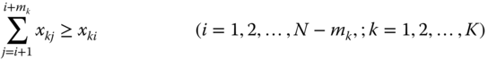
If xki = 0, then this constraint has no restriction. And if xki = 1, then at least one of ![]() must be equal to 1.
must be equal to 1.
- Let

Then we require that

If no maintenance is made in period i, then all xki = 0, so zi = 0. If at least one maintenance is done in period i, then ![]() , so zi must not be 0, and the right‐hand side of this inequality allows it to be equal to 1.
, so zi must not be 0, and the right‐hand side of this inequality allows it to be equal to 1.
- The maximum number of maintenance actions in each time period must not exceed M:
1.118

The objective function is to minimize the number of time periods when maintenance is done:

This problem is a linear binary optimization problem, which can be solved by routine methods.
We also might minimize the total cost:
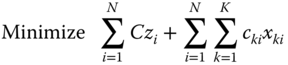
where C is the setup cost and cki is the maintenance cost of machine k in time period i.
A comprehensive summary of the most important maintenance models and methods is presented, for example, in (Valdez‐Flores and Feldman 1989), (Nakagawa 2006, 2008 ), (Jardine 2006), and (Wang 2002).
1.8.3 Condition‐Based Maintenance or Replacement
Next, we present a model of CBM or replacement if repair is not feasible or not economical (Hamidi et al. 2017). Consider a machine that produces utility with rate u(t) after t time periods of operation, which includes the value of its produced utility minus all costs of operation. Assume at time T a sensor shows the start of a degradation process, resulting in a decrease in utility production, in addition to increased operation and replacement costs because of the increased level of degradation. In formulating the mathematical model to find the optimal time of repair or replacement, the following notations are used:
- α = Degradation coefficient
- β = Cost of repair or replacement increase coefficient
- x = Planned time of repair or replacement
- u(t)e−α(t − T) = Density of utility value produced at time t > T
- Keβ(x − T) = Cost of repair or replacement at time x
So, the total net profit per unit time can be given as

which is maximized with respect to the decision variable x. Notice first that the derivative of g(x) has the same sign as

where

and G(x) tends to negative infinity as x converges to infinity.
Notice that
since u(x) is nonincreasing. So G(x) is a strictly decreasing function of x. Let T* > T be the latest time period when the repair or replacement must be performed.
So, we have the following three possibilities:
- G(T) ≦ 0. Then G(x) < 0 for all x > T, so g(x) decreases, and therefore T is the optimal x value.
- G(T*) ≧ 0. Then G(x) > 0 for all x < T*, so g(x) increases, and therefore T* is the optimum x value.
- Otherwise, G(T) > 0 and G(T*) < 0, and there is a unique
 such that
  . This
  value is the optimum scheduled repair or replacement time.
In cases where there are several machines with different parameters, and a common time x is to be determined to repair or replace them together in order to decrease setup costs, then Eq. (1.121) is generalized as

where the summation is made for all machines involved. Similar to the previous case, the derivative of g(x) has the same sign as

and furthermore

So, the optimum depends on the signs of G(T) and G(T*), as in the previous case.
Consider next the special case of one machine with u(t) ≡ u and β = 0: that is, a constant production rate and no increase in repair/replacement costs.
Then
If βT < 1, then the optimal time is larger than T.
1.8.4 Preventive Replacement Scheduling
The optimum timing of preventive replacement is next discussed. In the case of a failure, the unexpected timing and the possible additional damages make the replacement more expensive than a preventive replacement. If replacement is done early, then a useful time interval is lost; and if it is scheduled late, then failure might occur, with a high replacement cost and possible damages and accidents. In scheduling preventive replacement, several factors should be considered.
Let X denote the random variable representing the time to unrepairable failure, when the object must be replaced. The CDF, PDF, reliability function, and failure rate of X are denoted by F(t), f(t), R(t), and ρ(t), respectively. Let cp and cf denote the cost of preventive and failure replacements, respectively. Assume that the preventive replacement is scheduled at time T; then the expected replacement cost is cpR(T) + cfF(T), and the expected cycle length is given as ![]() , which can be rewritten as
, which can be rewritten as ![]() . If identical cycles repeat indefinitely, then the expected cost per unit time can be obtained based on the renewal theory as
. If identical cycles repeat indefinitely, then the expected cost per unit time can be obtained based on the renewal theory as

which is minimized (Barlow and Proschan 1965; Aven and Jensen 1999). In many cases – for example, in fast‐changing technologies – the optimum must be obtained based on the single‐cycle criteria. The cost per unit time is given as

with expected value

which is then minimized. In the case of several distribution types, the optimal solution can be obtained easily.
Consider first the model in Eq. (1.123). Its derivative has the same sign as

or

The derivative of the bracketed expression is
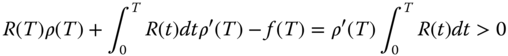
if ρ(T) is increasing. So Eq. (1.125) is an increasing function, and its value at T = 0 is −cp < 0. As T → ∞, it converges to infinity if ρ(T) → ∞ as T → ∞; otherwise it converges to a positive limit if

Therefore, in these cases there is a unique ![]() that makes Eq. ( 1.125
) 0, and this is the unique optimum. If the limit of Eq. ( 1.125
) is non‐positive at infinity, then there is no finite optimum, and the equipment must be replaced when it fails.
that makes Eq. ( 1.125
) 0, and this is the unique optimum. If the limit of Eq. ( 1.125
) is non‐positive at infinity, then there is no finite optimum, and the equipment must be replaced when it fails.
The derivative of Eq. (1.124) has the form
with the same sign as
If ρ(T) increases, then this function also increases; at T = 0, its value converges to −∞; and as T → ∞, its limit is positive. So, there is again a unique solution that is the unique optimizer. The solution of monotonic equations can be obtained by standard computer methods (Yakowitz and Szidarovszky 1989).
1.8.5 Model Variants and Extensions
There are many variants and extensions of these models. Some of them will be briefly introduced.
Assume first that preventive replacements need Tp time to perform and Tf is the same for failure replacements. If we consider a cycle until a replacement starts operating, then Tp or Tf must be included in the cycle length. Eq. ( 1.123 ) is modified as

and Eq. ( 1.124 ) becomes

These simple models do not take any additional elements into account: the cost of repairs of repairable failures, revenues generated by the product made by the machine, the salvage value after replacement, the optimal timing of the arrival of the spare parts, as well as the length of time required to perform repairs and the replacement. For the development of more advanced models, we introduce the following notations:
- cr = Cost of each repair
- M(T) = Expected number of repairable failures in interval [0, T]
- u(T) = Generated revenue in interval [0, T]
- S(T) = Salvage value of the equipment after lifetime T
- α = Unit inventory cost of spare part
- β = Unit loss of production delay
A new decision variable must be also included:
- W = Arrival schedule of spare part
For the sake of mathematical simplicity, we introduce the following function. If the equipment must be scheduled to be replaced at time t and the spare part arrives at time W, then the additional cost is

In the first case, an inventory cost occurs; and in the second case, a production delay causes losses to the company.
If long‐term expected costs are considered, then Eq. ( 1.124 ) is generalized as

and the corresponding one‐cycle model is extended to a more complicated objective function:

Both models have two decision variables, so for their optimization, commercial software is the best option. A complicated analytical approach is offered by the following idea. Consider first the value of T given, and optimize Eqs. (1.129) and (1.130) with respect to W. Clearly, the optimal W value depends on T : W = W(T). Then substitute W(T) into the objective functions, which now will depend only on T, so they become simple, single‐variable search algorithms that can be used to find the optimal solutions.
If short‐term and long‐term objectives are considered simultaneously, then a multi‐objective optimization method must be used with these two objective functions.
We can also incorporate the possibility of non‐repairable failures in Eqs. ( 1.121 ) and (1.122). In this case, the conditional CDF of TTF after time T must be used, which can be obtained as follows:

Notice that these objectives represent expected costs per unit time without considering their uncertainties, which are characterized by the variances of the costs per unit time. Both expected costs and their variances should be minimized, leading again to the application of multi‐objective optimization procedures.
A simple model is finally introduced to find the needed number of repair kits in any interval during the lifecycle of a piece of equipment. A similar model can be developed to plan the necessary amount of labor as well. For the sake of simplicity, assume that in cases of repairable failures, minimal repairs are performed. It is known from Section 1.5.1 that the number of failures in any interval [t, T] follows a Poisson distribution with expectation

meaning the times of failures form a non‐homogenous Poisson process. Assume that each repair requires one unit of repair kit. It is a very important problem to determine the number of units that guarantees that all failure repairs can be performed with at least a given probability value 1 − p. Let Q denote the required available number of kits; then with the notation
we require that

implying that

The required value of Q can be obtained by repeatedly adding the terms of the left‐hand side, starting with k = 0, until we reach or exceed (1 − p)eλ.
In more complicated cases, the same method as shown in Section 1.5.1 can be used to find the second moment of the number of failures; then its variance can be easily obtained. Let μ and σ2 denote the expectation and variance of the number of failures in interval [t, T]; then its distribution can be approximated by a normal distribution, and the condition from Eq. (1.133) is replaced by the following:

where φ(t) is a CDF. Therefore
where the smallest integer exceeding the right‐hand side gives the required number of repair kits.
1.9 Introduction to PHM: Summary
This chapter first gave a brief summary of reliability engineering and a probabilistic approach. It provided some statistical information about a large collection of identical items, which gives no information about a particular item. The different types of distributions of time to failure under normal or extreme stress conditions, the uncertainty of model parameters, and the expected number of failures with different types of repair or with failure replacement were discussed.
This introduction also provided a high‐level introduction to PHM, including the following topics: (i) traditional approaches to PHM‐enabling a system; (ii) DPS transfer curve and failure, and ideal and non‐ideal FFS transfer curves; (iii) data conditioning; and (iv) prognostic information. The chapter introduced some important prognostic parameters and a new performance metric: convergence efficiency. These topics are discussed in more detail in the following chapters of this book. This introductory chapter presented only a brief outline of material related to signatures, data conditioning, and prognostic information; that material will be elaborated on further in later chapters. In addition, a brief overview of the cost‐benefit analysis through the entire lifetime of equipment was provided.
References
- Arrhenius, S.A. (1889). Über die Dissociationswärme und den Einfluβ der Temperatur auf den Dissociationsgrad der Elektrolyte. Zeitschrift für Physikalische Chemie 4: 96–116.
- Aven, T. and Jensen, U. (1999). Stochastic Models in Reliability. New York: Springer.
- Ayyub, B.M. and McCuen, R.H. (2003). Probability, Statistics, and Reliability for Engineers and Scientists, 2e. Boca Raton: CRC Press.
- Barlow, R.E. and Proschan, F. (1965). Mathematical Theory of Reliability. New York: Wiley.
- Bucy, R.S. and Joseph, P.D. (2005). Filtering for Stochastic Processes with Applications to Guidance. Providence, RI: AMS Chelsea Publishing.
- Cox, D. (1970). Renewal Theory. London: Methuen and Co.
- Elsayed, E.A. (2012). Reliability Engineering. Hoboken, NJ: Wiley.
- Eyring, H. (1935). The activated complex in chemical reactions. The Journal of Chemical Physics 3 (2): 107–115.
- Finkelstein, M. (2008). Failure Rate Modeling for Reliability and Risk. London: Springer.
- Frieden, B.R. (2004). Science from Fisher Information: A Unification. Cambridge, UK: Cambridge University Press.
- Hamidi, M., Matsumoto, A., and Szidarovszky, F. (2017). Optimal schedule of repair or replacement after degradation is noticed. 46th Annual Meeting of the Western Decision Science Institute, Vancouver, Canada, 4–8 April.
- Hamilton, J. (1994). Time Series Analysis. Princeton, NJ: Princeton University Press.
- Hofmeister, J., Goodman, D., and Wagoner, R. (2016). Advanced anomaly detection method for condition monitoring of complex equipment and systems. 2016 Machine Failure Prevention Technology, Dayton, Ohio, US, 24–26 May.
- Hofmeister, J., Goodman, D., and Szidarovszky, F. (2017a). PHM/IVHM: checkpoint, restart, and other considerations. 2017 Machine Failure Prevention Technology, Virginia Beach, Virginia, US, 15–18 May.
- Hofmeister, J., Szidarovszky, F., and Goodman, D. (2017b). An approach to processing condition‐based data for use in prognostic algorithms. 2017 Machine Failure Prevention Technology, Virginia Beach, Virginia, US, 15–18 May.
- IEEE. (2017). Draft standard framework for prognosis and health management (PHM) of electronic systems. IEEE 1856/D33.
- Jardine, A. (2006). Optimizing maintenance and replacement decisions. Annual Reliability and Maintainability Symposium (RAMS), Newport Beach, California, US, 23–26 January.
- Kececioglu, D. and Jacks, J.A. (1984). The Arrhenius, Eyring, inverse power law and combination models in accelerated life testing. Reliability Engineering 8 (1): 1–9.
- Kumar, S. and Pecht, M. (2010). Modeling approaches for prognostics and health management of electronics. International Journal of Performability Engineering 6 (5): 467–476.
- Medjaher, K. and Zerhouni, N. (2013). Framework for a hybrid prognostics. Chemical Engineering Transactions 33: 91–96. https://doi.org/10.3303/CET1333016.
- Milton, J.S. and Arnold, J.C. (2003). Introduction to Probability and Statistics. Boston, MA: McGraw Hill.
- Mitov, K.V. and Omey, E. (2014). Renewal Processes. New York: Springer.
- Nakagawa, T. (2006). Maintenance Theory and Reliability. Berlin/Tokyo: Springer.
- Nakagawa, T. (2008). Advanced Reliability Models and Maintenance Policies. London: Springer.
- National Science Foundation Center for Advanced Vehicle and Extreme Environment Electronics at Auburn University (CAVE3). (2015). Prognostics health management for electronics. http://cave.auburn.edu/rsrch‐thrusts/prognostic‐health‐management‐for‐electronics.html (accessed November 2015).
- Nelson, W. (1980). Accelerated life testing – step stress models and data analysis. IEEE Transactions on Reliability R‐29 (2): 103–108.
- Nelson, W. (2004). Accelerated Testing: Statistical Models, Test Plans, and Data Analysis. New York: Wiley.
- O'Connor, P. and Kleyner, A. (2012). Practical Reliability Engineering. Chichester: Wiley.
- Pecht, M. (2008). Prognostics and Health Management of Electronics. Hoboken, NJ: Wiley.
- Pratt, J.W., Edgeworth, F.Y., and Fisher, R.A. (1976). On the efficiency of maximum likelihood estimation. Annals of Statistics 4 (3): 501–514.
- Ross, M.S. (1987). Introduction to Probability and Statistics for Engineers and Scientists. New York: Wiley.
- Ross, M.S. (1996). Stochastic Processes, 2e. New York: Wiley.
- Ross, M.S. (2000). Probability Models, 7e. San Diego, CA: Academic Press.
- Saxena, A., Celaya, J., Saha, B. et al. (2009). On applying the prognostic performance metrics. Annual Conference of the Prognostics and Health Management Society (PHM09), San Diego, California, US, 27 Sep.‐1 Oct.
- Speaks, S. (2005). Reliability and MTBF overview. Vicor Reliability Engineering. http://www.vicorpower.com/documents/quality/Rel_MTBF.pdf (accessed August 2015).
- Szidarovszky, F., Gershon, M., and Duckstein, L. (1986). Techniques of Multiobjective Decision Making in Systems Management. Amsterdam: Elsevier.
- Valdez‐Flores, C. and Feldman, R.M. (1989). A survey of preventive maintenance models for stochastically deteriorating single‐unit systems. Naval Research Logistics 36: 419–446.
- Wang, H.Z. (2002). A survey of maintenance policies of deteriorating systems. European Journal of Operational Research 139 (3): 469–489.
- Yakowitz, S. and Szidarovszky, F. (1989). An Introduction to Numerical Computations. New York: Macmillan.
Further Reading
- Filliben, J. and Heckert, A. (2003). Probability distributions. In: Engineering Statistics Handbook. National Institute of Standards and Technology. http://www.itl.nist.gov/div898/handbook/eda/section3/eda36.htm.
- Hofmeister, J., Wagoner, R., and Goodman, D. (2013). Prognostic health management (PHM) of electrical systems using conditioned‐based data for anomaly and prognostic reasoning. Chemical Engineering Transactions 33: 992–996.
- Tobias, P. (2003a). Extreme value distributions. In: Engineering Statistics Handbook. National Institute of Standards and Technology. https://www.itl.nist.gov/div898/handbook/apr/section1/apr163.htm.
- Tobias, P. (2003b). How do you project reliability at use conditions? In: Engineering Statistics Handbook. National Institute of Standards and Technology. https://www.itl.nist.gov/div898/handbook/apr/section4/apr43.htm.