Search in book...
Toggle Font Controls
Create new playlist

Name your new playlist

Playlist description (optional)
Sign In

Email address

Password

Forgot Password?

or

Continue with Facebook

Continue with Google
Sign Up

Full Name

Email address

Confirm Email Address

Password

or

Continue with Facebook

Continue with Google

3
Failure Progression Signatures

3.1 Introduction to Failure Signatures

Chapter 2 introduced three classical prognostic approaches for prognostics and health management/monitoring (PHM): model driven, data driven, and hybrid driven. You were also introduced to usage‐based and condition‐based approaches. You learned the primary disadvantages of classical and usage‐based approaches for prognostics: they are not applicable to a specific prognostic target in a system, and/or they are nondeterministic and not suitable for application to prognostic targets, and/or it is complex to adapt them to sensor data. You also learned that leading indicators of failure can be extracted from sensor data and collected to form condition‐based data (CBD) signatures; the modeling and processing of such signatures is a condition‐based approach to condition‐based maintenance (CBM). Figure 3.1 shows the relationship of an approach using CBD signatures to classical PHM approaches; although the block diagram indicates the approaches are different, a conditioned‐based approach often employs analysis and modeling techniques such as reliability modeling, physics of failure (PoF) analysis, and failure mode and effect analysis (FMEA) (Hofmeister et al. 2013, 2016, 2017; Medjaher and Zerhouni 2013; Pecht 2008).

Similar image as in Figure 2.12 with prognostic approaches also branching to a box for condition-based data (CBD) signatures. — Figure 3.1 Diagram of classical and CBD prognostic approaches for PHM systems.
Source: based on Pecht ( 2008 ).

3.1.1 Chapter Objectives

The primary objective of this chapter is to take a more in‐depth look at CBD signatures and the desirability of transforming those signatures into other signatures that are more amenable as input to prediction algorithms that produce prognostic information. Those other signatures are the fault‐to‐failure progression (FFP) signature, degradation progression signature (DPS), and functional failure signature (FFS).

A secondary objective is to describe and show how those signatures are used for reliable condition‐based monitoring: detecting the onset of degradation, monitoring the increasing progression of damage due to degradation, making prognostic estimates for when damage is likely to reach a level defined as functional failure, and detecting functional failure.

Another objective is to show an important advantage of DPS data and DPS‐based FFS compared to CBD signature or FFP signature curves: the former is more linear. A method for quantifying the nonlinearity of FFP‐based and DPS‐based FFS curves shall be developed and presented in this chapter.

3.1.2 Chapter Organization

The remainder of this chapter is organized to present and discuss a heuristic‐based approach to modeling CBD signatures as follows:

3.2 Basic Types of Signatures
This section presents information on basic types of signatures: CBD signatures, FFP signatures, FFP‐based FFS, transforming FFP signatures into DPS, and DPS‐based FFS.
3.3 Model Verification
This section discusses model verification along with signal classification and verifying CBD, FFP, DPS, and DPS‐based models.
3.4 Evaluation of FFS Curves: Nonlinearity
This section discusses the evaluation of FFS curves in the context of a transfer curve for a sensing system and how to calculate metrics that quantify the nonlinearity of that transfer curve.
3.5 Summary of Data Transforms
This section summarizes the material presented in this chapter.

3.2 Basic Types of Signatures

A signature characterizes a feature of interest, such as feature data (FD) amplitude with respect to time: signature = FD = a set of FD_i data points over a period of time T = {t_m, t_m + 1,…t_m + n}, where amplitude refers to a characteristic value such as voltage, current, resistance, force, energy, and so on that changes as the magnitude of damage/degradation increases over time:

3.1

There are three signatures of interest related to signals and prognostic processing: CBD, FFP, and DPS. An FFP signature is a transform of a CBD signature to reduce modeling complexity, and a DPS signature is a transform of an FFP signature that further reduces modeling complexity and lends itself to increased accuracy of prognostic information. Another signature is particularly amenable to processing by prediction algorithms: an FFS that is a transform of either an FFP or a DPS signature. We will next show how the different signatures can be obtained.

3.2.1 CBD Signature

As illustrated in Figure 3.2, a sensor is located at a node of prognostic interest, such as the output of a switch mode power supply (SMPS). The sensor is designed to capture and process CBD, such as that shown in Figure 3.3, to support the isolation and extraction of FD: a leading indicator of failure. Isolation and extraction of a particular value of FD, such as the resonant frequency of a damped‐ringing response of an SMPS to an abrupt change in output load, almost always requires signal conditioning. Signal conditioning includes, but is not limited to, the following: background noise and harmonic filtering and mitigation; gating of the signal to specific, timed events to sufficiently isolate a feature of interest; fusing of two or more signals to transform two types of data to another data type – such as using voltage and current signals to calculate impedance; domain transforms such as time‐to‐frequency and frequency‐to‐time; and fusing of signals to cancel or mitigate environmental variations such as resistive dependence on temperature. Chapter 5 provides more information on signal conditioning.

Functional block diagram for CBD signature data and processing flow, displaying a box containing graphs for monitored nodes with arrows leading to a graph of A vs. T having an ascending curve for CBD signature data. — Figure 3.2 Functional block diagram for CBD signature data and processing flow.

Graph of temperature vs. measurement time with a fluctuating curve, illustrating an example of CBD containing feature data and noise (FD+noise). — Figure 3.3 Example of CBD containing feature data and noise (FD + Noise).

A CBD data point in a leading indicator of failure comprises a feature of interest, FD, in a signal that changes as degradation progresses, plus all other variations, referred to as noise (N), that are not related to degradation and the feature of interest:

3.2

Signals at nodes within a system typically exhibit more than just a particular CBD of interest. An example of signals is shown in Figure 3.4; the node is the output of a SMPS, and a particular CBD of interest is a damped‐ringing response such as that shown in Figure 3.5, for which an idealized plot is shown in Figure 3.6 (Erickson 1999; Judkins et al. 2007; Judkins and Hofmeister 2007; Hofmeister et al. 2013 , 2016 , 2017 ).

Image described by caption and surrounding text. — Figure 3.4 Example of signals at an output node of an SMPS.

Graph of amplitude vs. time with a fluctuating curve, illustrating an example of a damped-ringing response. — Figure 3.5 Example of a damped‐ringing response (Judkins and Hofmeister 2007 ).

Graph of voltage vs. time displaying a sine waveform with decreasing amplitude, a dotted curve labeled e, dimensional arrows labeled AR and TR. — Figure 3.6 Modeling a damped‐ringing response.
Source: based on Judkins and Hofmeister ( 2007 ).

The signals shown in Figure 3.4 consist of multiple types of CBD and noise, including damped‐ringing responses, switching noise from power transistors, ripple voltage, pulse‐width modulator effects, effects of voltage and current regulation and feedback, and background noise:

3.3

where CBD_i are signal terms and N_j are noise terms. An example of a CBD term is a damped‐ringing response, such as that shown in Figure 3.5 . An idealized damped‐ringing response is shown in Figure 3.6 and is modeled as

which includes five possible features of interest: a direct current (DC) voltage V_DC, a response amplitude A_R, a dampening time constant τ, a frequency ω, and a phase shift φ.

Even noise, with appropriate signal conditioning and processing, can be used as CBD – for example, to prognostic‐enable a noise‐filtering subcircuit in an SMPS. The primary objective of sensors used in prognostic‐enabling applications is to isolate CBD that forms leading indicators of failure, which, after suitable signal conditioning, are transformed into FD in signatures for use as input to prediction algorithms.

Example 3.1

Suppose you have been asked to prognostic‐enable an SMPS used by a customer for two different applications: a high‐end application with conservative failure requirements and a low‐end application with less stringent failure requirements. You decide to select the resonant frequency of a damped‐ringing response (example presented in Chapter 2) as your leading indicator of failure: (i) loss of filtering capacitor is the predominant failure mode; (ii) therefore as the power supply degrades due to that loss, the resonant frequency increases; and (iii) changes in resonant frequency are less dependent on load changes compared to, for example, changes in amplitude of ripple voltage.

Starting with Eq. (2.49) and letting C₀ represent the value of an undamaged capacitor,

where frequency in Hz is given by

3.4

then the signal model becomes

3.5

where a scalar value of frequency, FD, is returned by an intelligent sensor attached to the output node of the SMPS. Then from Eqs. (3.2) and (3.5),

3.6

Figure 3.6 shows an idealized plot of a damped‐ringing response and features of interest such as the resonant frequency f_R = 1/T_R, which is related back to Eq. (3.4).

Example 3.3

Now that you have selected the feature of interest (frequency) and have a model, Eq. (3.1), you need to design a solution, develop a test bed, and complete a design of experiment(s) (DOE) to be used to verify your chosen solution. Referring back to Figure 3.1 , you determine that the PHM solution needs to handle the following variability in the data:

Noise, in the form of frequency variability (refer back to Figure 3.1 ).
The nominal value of frequency (FD₀) in the absence of degradation: ΔC = 0.
The frequency amplitude at which the SMPS is defined as functionally failed for the high‐end application and for the low‐end application.

As a result of interaction with customer representatives and engineers, you determine that your design and the technology you are using let you specify 0.6 kHz as a noise margin (NM) to mitigate unfiltered noise: 2.5% of the nominal value of 24 kHz as the resonant frequency of an average, undamaged SMPS. You also define the failure level (FL) for the high‐end application as a loss of 60% filtering capacitance and the FL for the low‐end application as a loss of 70% filtering capacitance.

Evaluation of the SMPS specifications indicates that manufacturing variations result in a resonant frequency that varies between 21 and 27 kHz. When you apply this information into a test‐bed design, build the test bed, execute your DOE, and collect experimental data, you end up with plotted results as shown in Figure 3.8 and the tabulated results shown in Table 3.1.

Figure 3.8 CBD signature and levels for SMPS lot 1 (top) and SMPS lot 2 (bottom).

Table 3.1 Range of failure thresholds: Lot 1 and Lot 2.

Boundary condition	High‐end failure level	Low‐end failure level
Lot 1: Nominal frequency 27 kHz	43.2	45.9
Lot 2: Nominal frequency 21 kHz	33.6	35.7

CBD Signature Evaluation

Evaluation of the CBD signature as input to an intended prediction algorithm leads to the following conclusions:

The prediction algorithm is likely to produce estimates of prognostic information – remaining useful life (RUL), state of health (SoH), and prognostic horizon (PH) – that meet the accuracy requirements of your customer, especially with regard to a required minimum prognostic distance (PD) within a specified accuracy (PD_α).
A large number of models are required to correctly process CBD signatures, especially in a large, complex system.
Using CBD signatures as an approach to PHM is perhaps as complex as classic model‐driven approaches.

3.2.2 FFP Signature

One way to simplify modeling is to normalize CBD signature data to create FFP signature data, and at the same time apply a noise margin to the data (see Figure 3.9). The procedure is to subtract from CBD an NM to create a FD_i value, then subtract a nominal FD₀ value and divide the result by the nominal FD₀ value:

3.7

Functional block diagram for FFP signature and processing flow, with 2 graphs of frequency vs. time and frequency ratio vs. time each displaying an ascending curve. — Figure 3.9 Functional block diagram for FFP signature and processing flow.

FFP signatures are preferable to CBD signatures because the effect of noise on prediction accuracy is mitigated by the use of a noise margin and because normalization results in relative units of measure in amplitude instead of units of measure such as kHz. Instead of a model for a nominal frequency of 24 kHz, a model for a nominal frequency of 24.3 kHz, a model for a nominal frequency of 24.6 kHz, and so on, you need only one model, which reduces both modeling and processing complexity when producing prognostic information.

Example 3.6

You realize that using a fixed value of 24 kHz as the nominal frequency introduces an offset type of error in the FFP signature data. From Table 3.1 , you realize that either you need to use 27 kHz or you need to use calibration. You evaluate your prognostic requirements and choose to employ the following in your design: (i) leave the design of the sensor as is, and (ii) employ a node‐based architecture that includes support for specifying a calibration phase in which a number of samples from the sensor are averaged, saved, and used as a nominal frequency. The bottom plot in Figure 3.10 shows the result of using a calibrated value of nominal frequency.

An FFP signature point at or below 0 in amplitude indicates no damage. A functional failure level is application‐dependent as illustrated by two functional failure thresholds: 0.6 for high‐end applications (top plot in Figure 3.11) and 0.7 for low‐end applications (bottom plot in Figure 3.11 ).

Figure 3.11 FFP signature, calibrated value for nominal frequency, failure threshold at 0.6 and 0.7.

FFP Signature: Nominal Value and Calibration for FD

As we have discussed, a prevailing problem with modeling data is variations in the data: signal‐induced noise, thermal‐induced noise, operational‐induced noise, environmental‐induced noise, manufacturing‐induced noise, and so on. A significant challenge in designing and developing PHM systems to achieve reliable conditioning monitoring is reducing and/or mitigating such variation to reduce the complexity in data processing to obtain affordable, reliable results. The previous example introduced complexity associated with the nominal value used to transform CBD signature data into FFP signature data: the nominal value for FD plus a noise margin must be equal to or greater than the maximum variation in data that results from manufacturing and all other variations in the data not associated with degradation.

There are two basic methods for determining the nominal value to use: (i) perform sufficient experiments, measurements, and analysis to make an accurate determination of the maximum value to use for all instantiations of a prognostic target; and/or (ii) perform a calibration step that sufficiently measures, calculates, and saves a nominal value to use for each instantiation. For applications requiring high precision and high accuracy in prognostic estimates, calibration may be best – otherwise, use high values.

FFP Signature Data: Failure Threshold

To use FFP signatures as input to a prediction algorithm, either models with a defined failure threshold need to be used, or the prediction algorithm must be told the value of the failure threshold.

FFP Signature Data: Benefits Compared to CBD Signature Data

FFP signatures require less modeling compared to CBD signatures: one model for each failure level compared to 20 models (refer back to 3.4). In addition, prediction‐algorithm processing of FFP signature data compared to that for CBD signature is greatly simplified:

An FFP point less than or equal to 0 represents a state of zero degradation: RUL = maximum (specified or system‐determined value) and SoH = 100%.
An FFP point between 0 and less than a specified failure threshold represents a degraded state: 0 < RUL < maximum and 0% < SoH < 100%.
An FFP point at or above a failure threshold represents a functionally failed state: RUL = 0 and SoH = 0%.

3.2.3 Transforming FFP into FFS

One technique for handling different levels/thresholds of functional failure is to divide FFP signature data by the value of the failure level (FL) and, at the same time, multiply the result by 100 to create FFS data related to percent of failure:

3.10

3.11

FFS Signature Data: Benefits Compared to FFP Signature Data

FFS signatures require the least modeling compared to CBD and FFP signatures: one model for all failure levels. In addition, prediction‐algorithm processing of FFS signature data is greatly simplified. Referring to Figure 3.12:

An FFS point less than or equal to 0 represents 100% health: RUL = maximum and SoH = 100%.
An FFS point greater than zero and less than 100 represents a degraded state: 0 < RUL < maximum and 0% < SoH < 100%.
An FFS point at or above 100 represents 0% health – that is, a functionally failed state: RUL = 0 and SoH = 0.

2 Graphs of FFS amplitude vs. time each with an ascending curve with a horizontal lien labeled zero degradation ← 0. Each graph has another horizontal line representing functional failure for FL = 0.6 and 0.7, respectively. — Figure 3.12 FFS signatures for FL = 0.6 (top) and FL = 0.7 (bottom).

Disadvantage of FFP‐Based FFS Data

A disadvantage of FFP‐based FFS data is that the signature is generally curvilinear: it has the same characteristic curve as the original CBD signature.

3.2.4 Transforming FFP into a Degradation Progression Signature (DPS)

The existence of a DPS that is a transform of an FFP signature has been asserted: now we present a general definition and a derivation of a particular FFP. We will also explain and demonstrate why a DPS approach to prognostic enabling for PHM is extremely advantageous compared to other CBD‐based approaches, including FFP and FFS for FFP signatures. Further, we have already explained and demonstrated that CBD‐based approaches are advantageous compared to classical model‐driven, data‐driven, and hybrid‐driven approaches to prognostic enabling for PHM.

Definition of a DPS

A DPS is a function of a change in value of a parameter of interest, dP:

When there is no degradation, the value of the parameter is unchanged and dP = 0.
As degradation progresses, the magnitude of dP increases.
3.12

Then defining dP_i to be an absolute value, dP_i = abs(dP_i), a particular DPS point becomes

3.14

Derivation of a DPS Model for an Exemplary FFP Signature

A derivation of a DPS model begins with the general model for a point in an FFP signature, Eq. ( 3.8 ),

to which we apply a model for an FD of interest, such as that for resonant frequency of a damped‐ringing response of an SMPS, Eq. ( 3.5 ):

Let P₀ = C₀ and dP_i = ΔC. Then

so that

Therefore,

and, rearranging terms,

And finally,

3.15

Comparison of DPS and FFP

A DPS is more linear compared to the FFP signature from which it is derived. When Eq. (3.15) is applied to an experimental‐based FFP signature, such as that shown in Figure 3.11 , the result is the DPS in the top plot of Figure 3.13. The comparison of both the DPS and its FFP is shown in the bottom plot.

Top: Graph of degradation ratio vs. time with an ascending curve labeled DPS: experimental data. Bottom: Graph displaying 2 ascending curves labeled DPS: experimental data and FFP: experimental data. — Figure 3.13 DPS and FFP signatures for data shown in Figure 3.11 .

Comparison of FFP‐Based and DPS‐Based Failure Thresholds

Comparing the DPS and FFP right‐side plots of Figure 3.13 indicates the amplitudes are different for a given point in time. This means an FFP signature at an amplitude ratio of 0.4 is not at the same level of degradation as for a DPS at that same amplitude ratio. This is because a failure level for an FFP signature is defined as follows:

3.16

Then from Eq. ( 3.8 ),

then

Then we have

And from Eq. ( 3.15 ),

3.17

Using a DPS‐Based Failure Level

Since an FFP signature is a FFP, it is logical to define a failure level using Eq. (3.16) and then calculate the equivalent level for dP/P₀ using Eq. (3.17).

3.2.5 Transforming DPS into DPS‐Based FFS

A DPS, similar to an FFP, is more useful when transformed into a DPS‐based FFS: divide DPS data signature data by the value of the failure level (FL) and, at the same time, multiply the result by 100 to create FFS data related to percent of failure:

3.18

3.19

Similar to an FFP‐based FFS, there is one model for all failure levels, and prediction‐algorithm processing of FFS signature data is greatly simplified.

3.3 Model Verification

It is important that all models used in a PHM system are verified: simulate each model, and compare the model against experimental and/or actual fielded data. There needs to be high correlation between the simulated data results and the results you obtain using experimental and/or field data. Most likely there will be discrepancies, but you should be able to explain those discrepancies to make an informed decision as to whether the discrepancies are acceptable and/or modeling and processing changes are necessary and/or desirable.

The verification focus of CBD modeling is comparing the characteristic curve exhibited by the CBD signatures against an ideal curve obtained from simulating your PoF‐based and/or FMEA‐based model. The objective of the modeling is not to exactly replicate CBD signatures with model‐simulated curves; rather, it is to ensure the totality of model‐simulated curves: the models for CBD signatures, FFP signatures, DPS data, and FFS data are sufficiently correlated and accurate. When FFS data is input to prediction algorithms in your PHM system, the resultant prognostic information needs to meet the accuracy, convergence, and reliability requirements for reliable condition‐based monitoring.

3.3.1 Signature Classification

There is little use for prognostic‐enabling a component that typically degrades from zero degradation (100% health) to functional failure (0% health) in less than a second. Instead, diagnostic detection, reporting, and remedial actions and/or disaster avoidance and/or remedial measures are really all that can be done for such “avalanche” failure modes. We are interested in degradation‐induced signatures: those signatures having changes that are highly correlated to the levels of degradation. Further, the time between the onset of degradation and a level of degradation that results in functional failure must be sufficiently long to enable the prognostic system to detect degradation, produce prognostic estimates that converge to a level of required accuracy, and do so on or before a required minimum length of time (a prognostic distance [PD]). We model signatures using the following general form we previously developed (Eq. (2.50) in Chapter 2):

3.20

where f(dP, P₀) is a degradation model, FD_i is a signature data point, FD₀ is the nominal value of a measurable feature absent any degradation, dP_i is a change in value of a parameter, and P₀ is the nominal value of that parameter absent any degradation.

As we shall see in this and the next chapter, the signature identification, conditioning, and transform methods used means it is not necessary to determine or use exact parameter values, but we need to identify the class of each signature to select a correct degradation model. The degradation‐related signatures result from failure modes that can be modeled as power functions or exponential functions.

Although degradation signatures are modeled as power functions or exponential functions that have either increasing or decreasing amplitudes, constant signatures are only applicable in the sense that they indicate the absence of degradation. We shall only use models for increasing amplitudes; signatures having decreasing amplitudes are transformed into a complementary, increasing‐amplitude signature and degradation model – more information on this is provided in the next chapter. Referring to Figures 3.16 and 3.17, degradation signatures are further classified by whether the signature has a decreasing or increasing slope angle as degradation progresses: a linear, straight‐line degradation signature is a special case that is classified as having a constant slope angle. The slope angle is the arc between a tangent to the curve and the horizontal axis.

2 Graphs of frequency vs. time each displaying 4 discrete ascending curves representing signatures with decreasing slope angles (top) and with increasing slope angles (bottom). — Figure 3.16 Examples of signatures: decreasing (top) and increasing (bottom) slope angles.

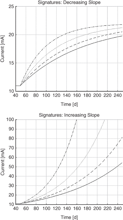
2 Graphs of current vs. time each displaying 4 discrete ascending curves representing signatures with decreasing slope angles (top) and with increasing slope angles (bottom). — Figure 3.17 Other examples of signatures: decreasing (top) and increasing (bottom) slope angles.

3.3.2 Verifying CBD Modeling

Verify that the model you have selected and/or developed is sufficiently correlated to the FD you have selected for processing. For example, when the system produces a signature that has a decreasing slope angle, your CBD modeling should produce a signature that has a decreasing slope angle, and both should have the same rate of change.

3.3.3 Verifying FFP Modeling

You need to verify your FFP modeling even when you do not intend to use FFP signatures. Your modeling should produce a characteristic FFP curve that is the characteristic CBD curve, except that the curve is shifted downward; it is at or below 0 in the absence of degradation; and the units of measure have changed from physical units such as voltage, amperes, and resistance to a ratio of values such as [voltage/voltage], and so on.

3.3.4 Verifying DPS Modeling

Similar to verifying FFP modeling, you need to verify your DPS modeling.

3.3.5 Verifying DPS‐Based FFS Modeling

A final step is to verify the model for a DPS‐based FFS.

3.4 Evaluation of FFS Curves: Nonlinearity

So far in this chapter, we have successfully developed and verified modeling to produce signatures:

FD_i = CBD_i – NM	Feature data point – Eq. (3.7)
FFP_i = (FD_i − FD₀)/FD₀	FFP signature point – Eq. (3.8)
DPS_i = 1 − (FD₀/FD_i)²	DPS point – Eq. (3.15)
FFS_i = 100 DPS_i/FL	FFS point (using DPS data) – Eq. (3.18)

The final transform uses Eq. (3.18) to produce a DPS‐based FFS to achieve an objective of transforming CBD signature data to FFS data: an ideal DPS‐based FFS is a straight line between the 0% and 100% data points. Prior to that, we developed a model, Eq. (3.10), for transforming FFP signature data into FFP‐based FFS data, and we made the following qualitative assessment:

A disadvantage of FFP‐based FFS data is that the signature is generally curvilinear: it has the same characteristic curve as the original CBD signature.

Figure 3.15 contains three plots of example FFS data: (i) a DPS‐based FFS, (ii) an ideal FFS transfer curve, and (iii) an FFP‐based FFS. A qualitative assessment of those curves might include the following:

The example DPS‐based FFS is more curvilinear compared to the ideal FFS.
The example FFP‐based FFS is also more curvilinear compared to the ideal FFS.
The example DPS‐based FFS is less curvilinear compared to the FFP‐based FFS.

But a visual inspection of the plots in Figure 3.15 indicates the latter qualitative assessment is not true for every data‐point‐by‐data‐point comparison of the DPS‐based FFS to the FFP‐based FFS. What we need is quantitative assessment – and we advocate a quantitative method for assessing the nonlinearity of FFS curves that is based on integral nonlinearity (INL) measurements that are commonly used for assessing the linearity of output‐transfer curves of data converters (Texas Instruments 1995; Carr and Brown 2000; Jenq and Qiong 2002).

3.4.1 Sensing System

A sensing system comprises everything between a monitored node and the input port of a predication system: the node, the sensor, and all the intervening frameworks. The prediction system acts upon the input from the sensing system to produce prognostic information used to provide a prognosis about a future failure: sensing hardware, data/domain converters, signal conditioning, data fusion, and so on.

In a PHM system, the sensing system provides input to a prediction system that processes the input from the sensing system to produce prognostic information that includes (i) RUL, (ii) SoH, and (iii) PH. An ideal RUL curve is a decreasing straight line between the point in time of the onset of degradation and the point in time of functional failure: the amplitude of that line is the time between functional failure and the onset of degradation. Similarly, an ideal SoH curve is a decreasing straight line between the point in time of the onset of degradation and the point in time of functional failure: an ideal SoH curve decreases linearly from 100% to 0% in amplitude. An ideal PH curve is a horizontal straight line comprising the sum of the current time of a sample and the RUL at that time.

The linearity of a sensing system is an assessment of how the measured curve produced by the sensing system deviates from the ideal curve (TI 1995 ; Carr and Brown 2000 ). The output of the sensing system is an FFS, and an ideal FFS input curve to the predication system is a straight line having a value of 0 just before the instant in time that degradation begins and a value of 100 at the instant when the monitored prognostic target is deemed to have functionally failed. For example, the left side of Figure 3.22 is a plot of an ideal FFS curve, and the right side of that figure is a plot of our example DPS‐based FFS; as shown, that curve deviates from an ideal FFS curve.

3.4.2 FFS Nonlinearity

We define functional‐failure signature nonlinearity (FNL) as a measure of the deviation between the actual FFS and an ideal FFS, very much like an INL assessment of an analog‐to‐digital data converter (ADC) or transducer output transfer curve (Texas Instruments 1995 ; Carr and Brown 2000 ; Jenq and Qiong 2002 ). A point‐by‐point FNL is a measurement of the error between an actual FFS value and the ideal FFS value at that point in time (see Figure 3.23). A total error (FNL_E) provides an assessment of the nonlinearity of the FFS curve (see Figure 3.24).

Graph of degradation vs. time displaying 2 ascending curves for DPS-based FFS and FFP-based FFS with 3 horizontal dashed lines delineating DPS-based FNLi and FFP-based FNLi. — Figure 3.23 Illustration of point‐by‐point FNL comparison.

Graph of degradation vs. time displaying 2 ascending curves for DPS-based FFS and FFP-based FFS with 3 ascending-horizontal dashed lines delineating DPS-based FNLE and FFP-based FNLE. — Figure 3.24 Illustration of total FNL_E comparison.

Calculating FFS Nonlinearity (FNL)

Calculating FNL is a post‐processing type of operation using FFS data, because we need to first calculate the total time between the point in time of the onset of degradation and the point in time when functional failure occurs:

3.21

Then for each point in the set {FFS_i}, we create an ideal point,

3.22

and calculate point‐by‐point nonlinearity,

3.23

and calculate total nonlinearity,

3.24

where max is a maximum function and abs is an absolute‐value function. Example plots on nonlinear errors are shown in Figure 3.25.

Graph of FNL error vs. time displaying 2 fluctuating curves for DPS-based FNLi (solid) and FFP-based FNLi (dotted). DPS-based FNLE of 13.1% and FFP-based FNLE of 16.9% are indicated. — Figure 3.25 Example plot of FFP‐based and DPS‐based *FNL*_i.

3.5 Summary of Data Transforms

Using an SMPS as an example, we described and showed the following signals and the transforms that were performed:

SMPS output (left side of Figure 3.26). Analog voltage of direct current (DC) and alternating current (AC) component features and noise. One of the features is damped‐ringing responses to abrupt changes in load.
Ringing response (right side of Figure 3.26 ). An intelligent sensor might do the following: present a series of abrupt, low‐power changes in load to the SMPS at timed intervals (sampling periods); capture the ringing responses; convert analog voltage to digital data; calculate an average frequency for each of several sinusoids in the response; calculate an average value of the average resonant frequency of each of the series of ringing responses; calculate the average frequency as a sample value; and output that average as a scalar CBD_i value.
CBD signature (left side of Figure 3.27). Sensor data is transformed into a CBD signature by subtracting the value of a noise margin from each received CBD_i to create a feature point, FD_i. The set of FD_i values, {FD_i}, is a CBD signature, as in Eq. ( 3.7 ):
FFP signature (right side of Figure 3.27 ). A set of FD_i values is transformed into a set of FFP_i values by subtracting from each FD_i value a nominal value of FD and dividing the result by that nominal value. The set of FFP_i values, {FFP_i}, is an FFP signature, as in Eq. (3.9):
FFP‐based FFS (left side of Figure 3.28). An FFP set, {FFP_i}, is transformed into {FFS_i} by dividing each value in the set by a functional‐failure level, FL, and multiplying the result by 100, as in Eq. ( 3.10 ):
DPS (right side of Figure 3.28 ). An FFP set, {FFP_i}, is transformed into {DPS_i} by transforming the FFP model into a new model that is a function of a parameter, P₀, and a change in that parameter, dP, and then solving for dP_i/P₀ in terms of the feature parameters FD_i and FD₀, as in Eq. ( 3.15 ):
DPS‐based FFS (Figure 3.29). A set of DPS values, {DPS_i}, is transformed into a DPS‐based FFS, {FFS_i} by dividing each DPS_i value in the set by an FL value and multiplying the result by 100, as in Eq. ( 3.18 ),
where FL is calculated using Eq. ( 3.17 ):

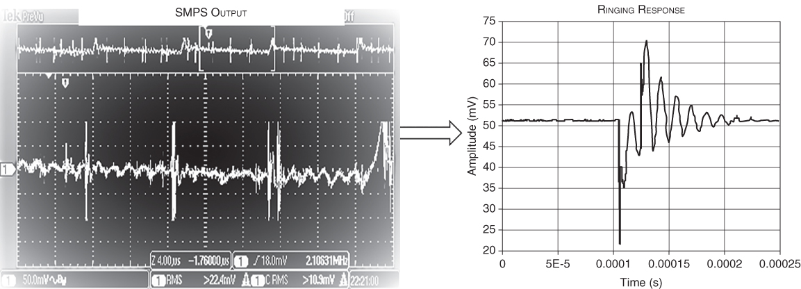
Graph displaying a fluctuating curve representing SMPS output (left) with an arrow pointing to a graph of amplitude vs. time with a fluctuating curve representing an extracted damped-ringing response (right). — Figure 3.26 SMPS output and extracted damped‐ringing response.

Graph of frequency vs. time with an ascending curve illustrating CBD signature (left) with an arrow pointing to a graph of frequency ration vs. time with and ascending curve illustrating FFP signature (right). — Figure 3.27 CBD signature and FFP signature.

Graph for FFP-based FFS, with a horizontal line labeled functional failure for FL = 0.7 intersected by an ascending curve for zero degradation ← 0, with right arrow to a graph for DPS data, with an ascending curve. — Figure 3.28 FFP‐based FFS and DPS.

Grap of degradation [%] vs. time [d] for DPS-based FFS, displaying an ascending waveform for FFS: Experimental CBD. — Figure 3.29 DPS‐based FFS.

High‐Level Procedure for Producing a DPS‐Based FFP

A high‐level procedure for producing a DPS‐based FFP is the following (refer to Figure 3.30): (i) select one or more output nodes to monitor for prognostic purposes; (ii) develop or acquire sensors to isolate CBD leading indicators of interest and to extract selected FD; (iii) signal condition and transform the collected FD to produce a CBD‐based signature – Eq. ( 3.6 ); (iv) further condition as necessary and transform CBD signature data into FFP signature data – Eqs. ( 3.7 ) and ( 3.8 ); (v) transform FFP signature data into DPS data using Eqs. ( 3.8 ) and ( 3.15 ); and (vi) transform DPS data into an FFS using Eqs. ( 3.17 ) and ( 3.18 ). You use Eqs. ( 3.21 )–( 3.24 ) to quantitatively assess the nonlinearity of FFS data.

Qualitative Assessment

The biggest advantage of the DPS approach is that DPS‐based FFS data is more linear compared to that based on FFP data. Additional advantages are the following:

Similar to an FFP signature, the amplitude of {DPS_i} data is dimensionless.
The number of required models is reduced.

Using Eq. (3.14) and the results of the examples used to verify modeling, we make the following inductive observations regarding the set {DPS_i}, regardless of the type of an underlying FD model (such as a linear or power function) and regardless of how FD changes with respect to time:

When a parameter dPi changes as a linear function with respect to time, {DPS_i} changes linearly with respect to time.
When a parameter dPi changes as a power function with respect to time, {DPS_i} changes as power function with respect to time.
When a parameter dPi changes exponentially with respect to time, {DPS_i} changes exponentially with respect to time.

The biggest advantage is the following: {DPS_i} is less curvilinear than its underlying {FFP_i} signature data, and so {DPS_i} data is particularly useful as input to prediction algorithms for processing to predict a future time of failure for a prognostic target.

3.6 Degradation Rate

In the previous section of this chapter, we saw that an ideal DPS‐based FFS is a linearly increasing line from 0 or less (no degradation) to 100 or more (functionally failed): an ideal DPS‐based FFS is a straight line between the 0% and 100% points. Even a non‐ideal DPS‐based FFS was shown to be less curvilinear than its underlying FFP signature (refer back to Figure 3.29 ). The linearity of a DPS‐based FFS is dependent on the linearity of the rate of change in a degrading parameter, dP: if the degradation rate with respect to time is constant, the DPS and the DPS‐based FFS will be linear; otherwise the degree of nonlinearity of the DPS and the DPS‐based FFS is dependent on the degree of nonlinearity in the degradation rate.

3.6.1 Constant Degradation Rate: Linear DPS‐Based FFS

As we have seen, an idealized DPS for a constant degradation rate results in an idealized linear DPS‐based FFS. And even when a DPS is not ideal, the DPS‐based FFS is more linear (less curvilinear) compared to the characteristic curve for its DPS. The examples and exemplary data we have been using are a result of assuming a constant degradation rate such as that modeled as follows:

3.25

in which δ = 1.0 for a constant degradation rate and t_i equals

3.26

where t_S is the time of a sample and t_D is the time of the onset of degradation: t_S ≥ t_D.

3.6.2 Nonlinear Degradation Rate

A non‐idealized DPS occurs when the degradation rate is not constant: it is nonlinear with respect to time. However, we will see that even when a DPS is not ideal, a DPS‐based curve is still more linear (less curvilinear) compared to its FFP signature.

Example 3.18

Plot a DPS, dP/P₀, using Eq. ( 3.25 ), where D₀ = 0.90/200 is valid after the onset of degradation, degradation begins at t = 51, and δ = 1.0 for a time period of 1 to 250 days. Compare the dotted‐line plot in Figure 3.31 to the solid‐line plot, in which dP = (0.75/200)t^1.05.

Figure 3.31 Linear DPS (left side) and nonlinear DPS (right side) data plots.

Notice that the differential nonlinearity (DNL) between the ideal, linear DPS and the non‐ideal, curvilinear DPS transfer curves is very small. The nonconstant degradation rate, in this case, increases the nonlinearity of the CBD and FFP signature curves from that seen on the left side of Figure 3.32. The nonlinearity increases even further, as shown on the right side of Figure 3.32 , when the nonlinearity in the degradation rate is increased even further: for example, to dP = (0.75/200)t^2.0.

Figure 3.32 Simulated CBD plots using nonlinear and linear degradation rates.

The DNL term introduced in 3.18 and a related term, integral nonlinearity (INL), are measurements of the deviation between two analog values: in this book, the two analog values are an ideal (straight line) signature and the signature of the data, such as an FFS, that is input to prediction algorithms (Texas Instruments 1995 ). In this book, we introduce a new term, FFS nonlinearity (FNL), which is a measurement of the deviation between ideal an RUL and an ideal SoH transfer curve and actual curves of the estimates of RUL and SoH from such prediction algorithms (Hofmeister et al. 2018).

3.7 Failure Progression Signatures and System Nodes

In Chapter 1, we used an example illustration of a framework for a PHM system for CBM. Referring to Figure 3.34, the framework comprises (i) a sensor framework, (ii) a feature‐vector framework, (iii) a prediction framework, (iv) a health‐management framework, (v) a performance‐validation framework, and (vi) a control‐ and data‐flow framework. The sensor framework is attached to a node, and in a system there might be hundreds or thousands of nodes, each of which is a point in a system that is a source of CBD: acoustic, electrical, magnetic, mechanical stresses and strains, vibration‐based, radiation, optical, and so on. It makes sense, then, to use a node‐based architecture as an anchor for a PHM system that collects CBD for reliable condition monitoring to support CBM.

Node-based framework for supporting failure progression signatures, with control & data flow framework linked to heath management, prediction, feature vector, performance validation, and sensor frameworks. — Figure 3.34 Node‐based framework for supporting failure progression signatures.

In this chapter, we presented and discussed sensors attached to nodes to monitor signals, to isolate CBD and FD using noise margins; calibration to use as nominal values for FD; and various transforms and data processing associated with CBD signatures, FFP signatures, DPS data, FFS data, and predications (prediction framework). It makes sense to use a node‐based architecture for a framework for a PHM system as opposed to, for example, designing and developing the details for each node in a control‐ and data‐flow framework. A sensor framework of sensors and drivers captures signals at nodes, performs data conditioning, and produces FD. A feature‐vector framework of processors performs additional conditioning and transforms to create FFSs used as input data to a prediction framework that produces prognostic information. A health‐management framework processes prognostic information to create diagnostic, prognostic, and logistics directives and actions to maintain the health and reliability of the system. A performance‐validation framework provides means and methods to produce prognostic‐performance metrics for evaluation of accuracy of prognostic information. A control‐ and data‐flow framework manages PHM functions and actions (CAVE3 2015; Hofmeister et al. 2017 ; Kumar and Pecht 2010; Pecht 2008 ).

3.8 Failure Progression Signatures: Summary

This chapter presented a rationale for transforming CBD signatures into other signatures: FFP, DPS, and FFS. You learned that both an FFP and a DPS can be transformed into an FFS. You saw that an FFP is a normalized version of a CBD and that an FFP greatly reduces the number of signature models; and we have shown that transforming an FFP into an FFS produces a very amenable signature for inputting to prediction algorithms:

Amplitude values are percentages.
Amplitudes of 0 or less indicate the absence of detection of degradation.
Amplitudes of 100 or greater indicate functional failure.

Functional failure is defined as a SoH condition in which a prognostic target is no longer operating within specifications.

You learned that you can transform an FFP into a DPS by solving the signature in terms of a change in a parameter value (dP) with respect to a nominal, non‐degraded value of the parameter (P₀): DPS = (dP/P₀); you also learned that a DPS is less curvilinear compared to an FFP and that there are two forms of DPS: constant and nonconstant degradation rate with respect to time:

You learned that a DPS, like an FFP, can be transformed into an FFS and that a DPS‐based FFS is most amenable to processing by prediction algorithms – even when the rate of degradation with respect to time is not constant.

You also learned that you need to verify your modeling choices against the signatures you are modeling and classify whether a signature has a decreasing or increasing slope angle as degradation progresses, to help determine the degradation function for a signature:

This chapter presented two quantitative measures for assessing the nonlinearity of an FFS curve: point‐by‐point nonlinearity and total nonlinearity, using Eqs. (3.23) and ( 3.24 ):

In the next chapter, you will learn that signatures can be effectively modeled by a limited number of characteristic curves: 10 power functions and 4 exponential functions. You will also learn that a heuristic approach to modeling signatures is sufficiently accurate for prognostics: formal modeling based on traditional methods such as FMEA and PoF is not necessary.

References

Carr, J.J. and Brown, J.M. (2000). Introduction to Biomedical Equipment Technology, 4e. Upper Saddle River, New Jersey: Prentice Hall.
Erickson, R. (1999). Fundamentals of Power Electronics. Norwell, MA: Kluwer Academic Publishers.
Hofmeister, J., Wagoner, R., and Goodman, D. (2013). Prognostic health management (PHM) of electrical systems using conditioned‐based data for anomaly and prognostic reasoning. Chemical Engineering Transactions 33: 992–996.
Hofmeister, J., Goodman, D. and Wagoner, R. (2016). Advanced anomaly detection method for condition monitoring of complex equipment and systems. 2016 Machine Failure Prevention Technology, Dayton, Ohio, US, 24–26 May.
Hofmeister, J., Szidarovszky, F., and Goodman, D. (2017). An approach to processing condition‐based data for use in prognostic algorithms. 2017 Machine Failure Prevention Technology, Virginia Beach, Virginia, US, 15–18 May.
Hofmeister, J.P, Goodman, D.L., and Szidarovszky, F. (2018). Transforming condition‐based data signatures into functional failure signatures, IEEE 2018 Aerospace Conference, Big Sky, Montana, US, 3–9 March.
Jenq, Y.C. and Li, Q. (2002). Differential non‐linearity, integral non‐linearity, and signal to noise ratio of an analog to digital converter. Portland, Oregon: Department of Electrical and Computer Engineering, Portland State University.
Judkins, J.B. and Hofmeister, J.P. (2007). Non‐invasive prognostication of switch mode power supplies with feedback loop having gain, IEEE Aerospace Conference 2007, Big Sky, Montana, US, 4–9 Mar.
Judkins, J.B., Hofmeister, J., and Vohnout, S. (2007). A prognostic sensor for voltage regulated switch‐mode power supplies. IEEE Aerospace Conference 2007, Big Sky, Montana, US, 4–9 Mar, Track 11–0804, 1–8.
Kumar, S. and Pecht, M. (2010). Modeling approaches for prognostics and health management of electronics. International Journal of Performability Engineering 6 (5): 467–476.
Medjaher, K. and Zerhouni, N. (2013). Framework for a hybrid prognostics. Chemical Engineering Transactions 33: 91–96. https://doi.org/10.3303/CET1333016.
National Science Foundation Center for Advanced Vehicle and Extreme Environment Electronics at Auburn University (CAVE3). (2015). Prognostics health management for electronics. http://cave.auburn.edu/rsrch‐thrusts/prognostic‐health‐management‐for‐electronics.html (accessed November 2015).
Pecht, M. (2008). Prognostics and Health Management of Electronics. Hoboken, New Jersey: Wiley.
Texas Instruments. (1995). Understanding data converters. Application Report SLAA013.