Search in book...
Toggle Font Controls
Create new playlist

Name your new playlist

Playlist description (optional)
Sign In

Email address

Password

Forgot Password?

or

Continue with Facebook

Continue with Google
Sign Up

Full Name

Email address

Confirm Email Address

Password

or

Continue with Facebook

Continue with Google

5
Non‐Ideal Data: Effects and Conditioning

5.1 Introduction to Non‐Ideal Data: Effects and Conditioning

Condition‐based data (CBD) contains feature data (FD) that forms signatures that are highly correlated to failure, damage, and degradation – especially fatigue damage due to the cumulative effects of stresses and strains induced by temperature, voltage, current, shock, vibration, and so on. Those signatures form curves that are not ideal, such as that shown in Figure 5.1; instead, CBD‐based signatures contain noise, they are distorted, and they change in response to that noise. That non‐ideality, when fault‐to‐failure progression (FFP) signatures are transformed into degradation progression signatures (DPS) and then into functional failure signatures (FFS), results in a non‐ideal transfer curve and errors in prognostic information. Those errors include the following: (i) an offset error between the time when degradation begins and the time of detection of the onset of degradation; and (ii) nonlinearity errors that reduce the accuracy of estimates of remaining useful life (RUL), state of health (SoH), and prognostic horizon (PH) – or end of life (EOL).

Graph of ratio vs. time displaying an ascending waveform for FFP: Experimental data intersected by an ascending curve for FFP: Simulated data. — Figure 5.1 Example of a non‐ideal FFP signature and an ideal representation of that signature.

5.1.1 Review of Chapter 4

Chapter 4 presented a set of seven signature models that resulted in FFP signatures having ideal, characteristic curves, such as those plotted on the top of Figure 5.2. Those ideal signatures were transformed into ideal DPS transfer curves of straight lines starting at an origin of 0 amplitude and passing through another data point having an amplitude of 1, such as those plotted on the bottom of Figure 5.2 . Two signatures are shown on the top of Figure 5.3: a curvilinear FFP signature and its transform into a linear DPS. That DPS was transformed into the FFS shown on the bottom of Figure 5.3 ; that FFS is a transfer curve that is very amenable to processing by a prediction system to produce prognostic information.

2 Graphs of FFP (top) and DPS (bottom) amplitude, each displaying 4 discrete lines representing P0=50, P0=75, P0=100, and P0=150. — Figure 5.2 Plots of a family of FFP signatures and DPS transfer curves.

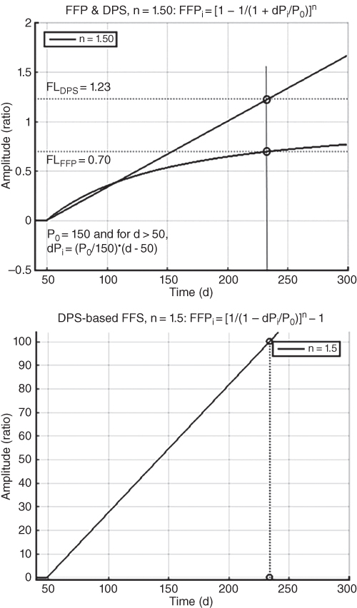
Image described by caption and surrounding text. — Figure 5.3 Plots of a curvilinear FFP, the transform to a linear DPS (top), and the transform to an FFS (bottom).

5.1.2 Data Acquisition, Manipulation, and Transformation

In this chapter, we continue an offline phase of developing models and methods: those oriented toward addressing nonlinearity effects due to noise. We use examples and descriptions to illustrate commonly encountered causes and effects of noise on the quality of data and on the nonlinearity of the final transfer curve – an FFS – of a sensing system. We present methods you might use to mitigate and/or ameliorate nonlinearity that prevents your sensing solution from meeting accuracy, resolution, and precision requirements.

In this book, we are not interested in how to prevent or avoid noise when designing and developing systems; rather, we are concerned with mitigating the effects of noise after data is collected by sensor frameworks, especially the effects of such noise on the linearity of the transfer curve of FFS data. Non‐ideality of that transfer curve, not the prediction algorithms, is the largest factor in the relative accuracy of prognostic information. We shall focus on the following three major processes:

Acquiring and manipulating data to improve the quality of data: removing and mitigating noise to a level sufficient to meet requirements related to prognosis accuracy.
Transforming data to form signatures that are amenable to prediction processing to produce prognostic information within accuracy requirements: attaching a sensing system to a node with the expectation that in the absence of degradation, data acquired and manipulated at that node will show neither a decreasing nor an increasing signature.
Modeling degradation signatures and signal‐conditioning methods in an offline phase, and then using those models and methods in an online phase to support the transformation of data into an FFS: transforming curvilinear, noisy CBD‐based signatures into linear, almost noiseless straight‐line transfer curves.

In Chapters 3 and 4, we used the resonant frequency of a damped‐ringing response of a switched‐mode power supply (SMPS) as the feature of interest. In this chapter, we shall discuss the amplitude of the ripple voltage at the output node of a SMPS as the feature of interest. The base set of models and methods to process signatures was completed in Chapter 4.

5.1.3 Chapter Objectives

CBD‐based signatures are not ideal: instead, they contain noise, they are distorted, they contain errors, and so on. Although we may have, for example, an intelligent sensor that is robust enough to attach to the output node of an SMPS – to sample data; perform Bessel, Butterworth, or Chebyshev filtering; digitize analog data; perform digital signal processing; and extract a condition indicator such as the amplitude of the ripple voltage (V_R, a type of FD) at the output node of that SMPS – we might discover that our signature is so noisy, it cannot be used without further signal conditioning.

A heuristic‐based approach to non‐ideal CBD signatures for prognostics and health management/monitoring (PHM) can be described as comprising four major processes in an offline and an online phase, as illustrated in Figures 5.4 and 5.5 (IEEE 2017; Medjaher and Zerhouni 2013):

Acquire and manipulate data to improve the quality of the data.
Transform the data to form signatures that are amenable to prediction processing to produce prognostic information within accuracy requirements.
Model degradation signatures and signal‐conditioning methods in an offline phase, and then use those models and methods to support the transformation of data into an FFS.
Process transformed data to produce prognostic information.

Sensing system offline phase diagram displaying boxes for monitor data, create models and methods, etc., a cylinder labeled Library: Models Methods, and a rightward arrows with labels data quality, conditioning, etc. — Figure 5.4 Offline phase to develop a prognostic‐enabling solution of a PHM system.

Diagram of an online phase to exploit a prognostic-enabling solution displaying boxes labeled monitor data, use models and methods, etc., with a rightward arrow with label data acquisition. — Figure 5.5 Diagram of an online phase to exploit a prognostic‐enabling solution.

In this chapter, we shall use the models (process #3) developed in Chapter 4 to transform exemplary data (process #2) to demonstrate causes and effects that reduce the quality of signatures (process #1), which reduces the accuracy of prognostic information (process #4). The objectives are to present and discuss sources of errors, significant effects of those errors on signatures, and methodologies and techniques that, when employed, ameliorate and/or mitigate errors by removing, reducing, and/or by avoiding such causes and effects. The goal is to improve the linearity and accuracy of FFS data used as input to the prediction system of a PHM system and, in doing so, improve the accuracy of prognostic information used to provide a prognosis of the health of the system being monitored and managed.

We shall apply a heuristic‐based approach to an example of a prognostic‐enabled component of an assembly in a system that, when subjected to degradation leading to failure, produces noisy CBD. That example will be an SMPS in which the capacitance of the output filter is reduced as degradation proceeds. The purposes include the following: (i) illustrate nonlinearity errors related to noise; (ii) identify, list, explain, and demonstrate some of the more common causes and effects leading to nonlinearity errors; and (iii) present and show methodologies that ameliorate and/or mitigate non‐ideality and/or the effects of non‐ideality.

5.1.4 Chapter Organization

The remainder of this chapter is organized to present and discuss topics related to the cause and effect of non‐ideality in signatures that result in nonlinearity errors. We present and discuss various methods and techniques to ameliorate and mitigate those effects:

5.2 Heuristic‐Based Approach Applied to Non‐Ideal CBD Signatures
This section summarizes a heuristic‐based approach for application to CBD signatures through the use of examples. Noise is identified as an issue in achieving high accuracy in prognostic information.
5.3 Errors and Non‐Ideality in FFS Data
This section presents and discusses topics related to nonlinearity, such as noise margin and offset error; measurement error, uncertainty, and sampling; other sources of noise; and data smoothing and non‐ideality in FFS data.
5.4 Heuristic Method for Adjusting FFS Data
This section describes a method for adjusting FFS data, adjusted FFS data, and data‐conditioning another example data set.
5.5 Summary: Non‐Ideal Data, Effects, and Conditioning
This section summarizes the material presented in this chapter.

5.2 Heuristic‐Based Approach Applied to Non‐Ideal CBD Signatures

CBD signatures are not ideal: they contain offset errors, distortion, and noise – including signal variations due to, for example, feedback effects and multiple failure‐mode effects. Included in this chapter are methods for mitigating and/or ameliorating such non‐ideality. Other errors are introduced in the processing of CBD signatures and the transformation of those signatures into FFS used as input to a prediction system.

Even if CBD was totally absent of noise and variability not related to degradation, attaching a sensor to a node to collect data and then processing that data introduces error into the data. Sensors may perform noise filtering or data sampling, or act as analog‐to‐digital data converters (ADCs), and digitized data is processed using digital signal processing (DSP) methods and techniques to include additional filtering, data fusion, data and domain transforms, data storage, and data transmission, all of which introduce errors into the data. Operational and environmental variability, such as voltage and temperature variability, are also sources of signal variability that result in non‐ideal data (Texas Instruments 1995; Jenq and Qiong 2002; Hofmeister et al. 2013, 2016, 2017).

5.2.1 Summary of a Heuristic‐Based Approach Applied to Non‐Ideal CBD Signatures

Chapter 4 presented a representative set of increasing FFP signatures: the negative of a decreasing signature produces an increasing signature. This chapter uses an approach that is summarized as follows and that we shall apply to non‐ideal CBD signatures (an example is shown in Figure 5.6):

Select a target within a system to prognostic enable, such as a component or assembly. The component should have a sufficiently high rate of failure and sufficient negative consequences related to failure to justify the costs of prognostic‐enabling that target.
Design and perform experiments that replicate degradation leading to the failure of interest and that produce CBD from which one or more candidate features of interest can be isolated and extracted. Evaluate those candidates, and reduce the set, preferably to three or less.
Characterize those CBD features as condition indicators, leading to one or more CBD signatures correlated to increasing degradation. Evaluate the signatures, and reduce the number of features to one or two candidates.
Convert an exemplary decreasing CBD signature to an increasing CBD signature.
Transform an exemplary increasing CBD signature into an FFP signature.
Analyze and characterize the exemplary FFP signature as one or more degradation signatures of a set of known signatures in a library of models:
- As necessary, develop a model for a new degradation‐signature model using a method similar to that used in Chapter 3.
- In this book, we will not develop any degradation‐signature models beyond the seven developed in Chapter 4.
Transform the exemplary FFP signature data into a DPS.
Transform the exemplary DPS into an FFS.
Perform experiments, collect new data, apply a set of sensing solutions, and evaluate the nonlinearity of the exemplary FFS. Choose the most promising set of solutions.
Select appropriate data‐conditioning methods to sufficiently reduce nonlinearity to meet requirements regarding accuracy, resolution, and precision of any prognostic estimates produced using the FFS. Assume the prediction system of the PHM system will not introduce further nonlinearity errors.
Adapt and implement data‐conditioning steps, such as those just described, to provide a solution in the frameworks of the sensing system of the PHM system. The solution includes the sensor and all firmware and/or software computational routines necessary to acquire and manipulate CBD signatures used to detect, isolate, and identify states related to health of the system; see Figures 1.1 and 1.2 in Chapter 1 (Carr and Brown 2000; Hofmeister et al. 2013 ; CAVE3 2015; IEEE 2017 ).

Image described by caption. — Figure 5.6 Plot of a non‐ideal CBD signature data: noisy ripple voltage, output of a switched‐mode regulator.

5.2.2 Example Target for Prognostic Enabling

For illustrative purposes, the capacitance of the output filter of an SMPS is selected as the prognostic target, and the output ripple voltage is selected as the CBD feature to be extracted as a condition indicator and processed as a signature. That power supply uses a design incorporating a sufficiently large value of output filtering capacitance that the amplitude of the ripple voltage is dependent on the resistivity of the load and not on the amount of filtering capacitance. Degradation effects that result in the loss of filtering capacitance will cause the amplitude of the output ripple voltage to increase (Erickson 1999; Judkins et al. 2007; Singh 2014).

Acquire Data, Transform It, and Evaluate It Qualitatively

We begin the process of prognostic‐enabling the SMPS by running experiments that inject faults and capture data. We verify that degrading the filter capacitance results in ripple voltage like that shown in Figure 5.6 : the signature is noisy and clearly not an ideal curve. The exemplary set data is a derived from actual experimental data; additional data points have been added, times were changed from minutes (an accelerated test) to hours, and noise amplitudes were changed for illustrative purposes. The signature results from a square root (n = 0.5) power function #3 type of degradation.

Example 5.1

Apply the modeling we have developed to the exemplary data shown in Figure 5.6 , and comment on the results:

From the shape of the curve, and using Table 4.2 in Chapter 4:

FFP‐signature model:	[1/(1 − dP_i/P₀)]ⁿ − 1
FFP‐to‐DPS transform model:	1 − 1/(FFP_i + 1)^1/n
FL transform from FFP‐based to DPS‐based:	1 − 1/( FL_FFP + 1)^1/n

The nominal value of the ripple voltage is 99.3 mV (FD₀ = 99.3 mV): calculated average of 10 samples prior to onset of degradation.
Use 0 for the noise margin (NM = 0 mV).
Define functional failure as FL_CBD = 250 mV, when CBD equals 250 mV.
Injected degradation for the experiment began when time equaled 98 hours.
Experimental data showed that CBD amplitude of 250 mV occurred when time equaled 153 hours.

First, transform the CBD‐based signature into an FFP signature, combining Eqs. (3.8) and (4.3) with the result shown on the top of Figure 5.7:

5.1

Figure 5.7 Example plots: non‐ideal FFP signature data (top) and transformed DPS data (bottom).

Then transform the FFP signature data into DPS data using the FFP‐to‐DPS transform model, and plot it as shown on the bottom of Figure 5.7 . From the specification of FL_CBD = 250 mV (functional failure), calculate FL_FFP

which you use to calculate FL_DPS:

to create FFS data that is plotted with the result shown on the top of Figure 5.8. An ideal FFS plot is also included on the bottom of Figure 5.8 . A qualitative comparison of the FFS data to the plotted ideal FFS appears favorable – although the data for times <100 hours is questionable, since that data indicates the presence of degradation.

Figure 5.8 Example plots: non‐ideal and ideal FFS data (top) and FNL (bottom).

Evaluate Data Quantitatively

Because an ideal FFS is a straight‐line transfer curve, a quantitative evaluation of results is possible by employing the FFS nonlinearity (FNL) method from Chapter 3. You decide it would be informative to calculate the positive nonlinearity, negative nonlinearity, and total nonlinearity:

5.2

5.3

5.4

Table 5.1 lists the steps in a procedure to quantitatively evaluate the nonlinearity of an FFS.

Table 5.1 FFS nonlinearity procedure.

Procedure name	Procedure expression
Calculate time to failure (TTF)	TTF = t_FA1LURE — t_0NSET
Create set of ideal data {lDEAL_FFS_i}	IDEAL_FFS_i = 100 (t_i – t_0NSET)/TFF
Calculate point‐by‐point nonlinearity {FNL_i}	FNL_i = FFS_i – IDEAL_FFS_i
Calculate positive nonlinearity (FNL_P)	FNL_P = max({FNL_i})
Calculate negative nonlinearity (FNL_N)	FNL_N = min({FNL_i})
Calculate total nonlinearity error (FNL_E)	FNL_E = FNL_P – FNL_N

Example 5.2

Perform an FNL procedure as outlined in Table 5.1 , and then plot and evaluate the results. Assume the following:

The desired FFS nonlinearity is to be within ±10% (PD_α = PD₁₀), on or before 75% of the maximum prognostic distance (PD), which is known from the experiment to be 155 hours starting at the onset of degradation (98 hours) and ending at functional failure (253 hours).
The desired FFS nonlinearity is to be within 5% (PD_α = PD₁₀), on or before 50% of the maximum PD.
No positive FFS nonlinearity prior to onset of degradation.

The nonlinearity of the FFS data on the left in Figure 5.8 is calculated and plotted on the right in Figure 5.8 . Table 5.2 lists the quantitative calculations, specifications, and results and evaluation. The evaluation is, “requirements are not met” – as indicated in the far‐right column of the table.

Table 5.2 List of calculations, specifications, and results for Example 5.2.

Name Maximum PD	Calculation/Specification PD = TTF = 155 hours	Required N/A	Result → Criteria
PD within 10%	PD1_10% = 100 (PD – PD₁₀)/PD	75%	PD₁₀ at 34.5 h 77.7% → met
PD within 5%	PD_5% = 100 (PD – PD₅)/PD	50%	PD₅ at 109.5 h 29.4% → did not meet
FNL_P	FNL_P = max({FNL_i})	N/S	10.0%
FNL_N	FNL_N = min({FNL_i})	N/S	−10.0%
FNL_E	FNL_E = FNL_P – FNL_N	N/S	20.0%
FNL_P	Before onset of degradation	0%	∼5% → did not meet

N/A, not applicable; N/S, not specified.

You conclude that the results did not meet requirements because of the effects of unmitigated noise in the data (see Figure 5.8 ) prior to the onset of degradation at 100 hours.

Example 5.3

Since the CBD‐based signature indicates the presence of noise of about 2 mV, it would be reasonable to use an NM of 3.0 mV, which equals the noise plus a 50% margin (contingency). Perform the transforms, the FNL procedure, and evaluations described in Examples 5.1 and 5.2 .

Using NM = 3.0 mV leads to one significant improvement: degradation is no longer detected (FFS_i > 0) prior to the actual time of the onset of degradation (98 hours). Instead of an early‐detection error, degradation is now detected at a later time (103.75 hours), and functional failure is detected at 253.75 hours. The offset error of 5.75 hours in the detection of the onset of degradation causes other changes in calculations: compare the plots in Figure 5.8 (NM = 0 mV) to the plots in Figure 5.9 (NM = 3.0 mV). Table 5.3 lists the results and indicates whether the result was a positive improvement (P) or a negative change (N).

Figure 5.9 Example plots: non‐ideal and ideal FFS data (top) and FNL (bottom) after using a NM of 3.0 mV.

Table 5.3 List of calculations, specifications, and results for Example 5.3.

Name	Calculation/Specification	Required	Result	Chg.
Maximum PD	PD = TTF = 151.25 h	N/A
PD within 10%	PD1_10% = 100(PD – PD₁₀)/PD	75%	PD₁₀ at 65 h 57.7% → did not meet	N
PD within 5%	PD_5% = 100 (PD – PD₅)/PD	50%	PD₅ at 105.0 h 30.6% → did not meet	P
FNL_P	FNL_P = max({FNL_i})	N/S	8.4%	P
FNL_N	FNL_N = min({FNL_i})	N/S	−14.0%	N
FNL_E	FNL_E = FNL_P – FNL_N	N/S	22.4%	N
FNL_P	Before onset of degradation	0%	0% → met	P

N/A, not applicable; N/S, not specified.

5.2.3 Noise is an Issue in Achieving High Accuracy in Prognostic Information

As we have just discussed, noise is an issue in achieving high accuracy in prognostic information: errors in the FFS data that is input to a prediction system are very likely to cause corresponding errors in the prognostic information. Example 5.2 illustrated two types of error: (i) false detection of degradation in the absence of detection and (ii) failure to meet PD requirements at a 5% level of accuracy. Example 5.3 illustrated that using a mitigation method, such as NM, introduces other forms of error such as a reduction in PD and an increase in nonlinearity.

Before making further attempts to ameliorate and/or mitigate the effects of noise, you need to understand the sources and effects of noise. Further, note that by “ameliorate and/or mitigate the effects of noise,” we are referring to solutions to be exploited after data is collected and processed by a sensor framework within the sensing system – we are not referring to solutions to reduce noise within the monitored system.

5.3 Errors and Non‐Ideality in FFS Data

In this section, we present topics related to noise: its sources and effects, and methods to ameliorate and/or mitigate errors and noise in FFS data. Noise, in the context of this book, is any unwanted signal or measurement that is not related to degradation: a specific failure mode or increasing level of damage. The topics presented include but are not limited to the following:

Noise margin and offset error
Measurement error, uncertainty, and sampling
Operating and environmental variability
Nonlinear degradation
Multiple modes of degradation

Most errors and noise in FFS data are the result of noise in the original signal at monitored nodes. Some errors and noise are introduced by hardware, firmware, and software used to acquire, manipulate, and store and retrieve data; other errors and noise are introduced by the solutions employed to ameliorate and/or mitigate noise and the effects of noise (Stiernberg 2008; Vijayaraghavan et al. (2008).

It should be understood that due to expense, in terms of both time and money, it is not possible to ameliorate all forms of noise. In addition to expense, there are operational limitations: often, if not invariably, ameliorating noise results in an increase in the weight of the solution(s) and an increase in the power to drive the solution(s). Therefore, mitigation methodologies are often used when, for whatever reason, amelioration methodologies are deemed too expensive and noise is evaluated as being unacceptably high.

A most important consideration is the following: it is not necessary to eliminate and/or mitigate all sources and effects of noise. Instead, eliminate, reduce, and/or mitigate appropriate and sufficient sources and effects of noise to meet the accuracy requirements related to the prognostic target.

The topics presented in this section include commonly encountered sources of variability that contribute to noise, such as the following:

Variability due to quantization error and other errors related to digitization.
Variability due to measurement errors related to sampling.
Variability due to the operating and ambient environments, including switching effects (spikes, glitches, and notches) and environmental effects (temperature, pressure, airflow, and so on).

We could, but will not, devote this entire book to noise and errors that ultimately result in noise, the sources of noise, and actions to address issues due to noise. Instead, we shall focus on noise that results in accuracy issues you are likely to encounter.

5.3.1 Noise Margin and Offset Errors

A commonly used mitigation method is an NM, such as that in Eq. (5.1), but using an NM or other mitigation method often introduces other errors. A primary error related to NM is an offset error in detecting the time of the onset of degradation:

5.5

This can be expressed as a percentage error related to estimated prognostic distance,

5.6

5.7

where t_FF is the time when functional failure is detected, and t_DETECT is when degradation is detected

5.8

where t_EOL is the true end of life or time of functional failure, and t_ONSET is the true time of the onset of detection. The error in prognostic distance is given by

5.9

Example 5.4

Using the data and results of Examples 5.2 and 5.3 , calculate the offset and PD errors introduced by the NM value used in Example 5.3. From the data and from Eq. (5.8),

After the NM is used, the estimated PD and error are calculated using Eqs. (5.7) and (5.9)

resulting in a 2.5% error. The offset error is calculated using Eqs. (5.5) and (5.6):

An important objective in achieving high accuracy and reliability in prognostic information is to reduce NM to the smallest value necessary to reliably prevent false detection of degradation and, at the same time, reduce the level of introduced errors. Invariably, to do so, you need to consider other methods to ameliorate and/or mitigate noise and its effects, and that means you must be aware of commonly encountered sources of noise and effects introduced by the sensing system and the pros and cons of solutions you might consider employing in the sensing system. The system being monitored is not subject to being improved by the sensing or prediction systems of a PHM system.

5.3.2 Measurement Error, Uncertainty, and Sampling

Measurement error, uncertainty, and sampling involve the monitoring, acquisition, manipulation, and storage and retrieval of data at points where noise and the effects of noise can be amplified and/or injected into signals. You need to take this into consideration when designing, developing, and evaluating a sensing system.

We shall use two cases as examples: one is a sensor that samples a signal at a node, digitizes the voltage, performs DSP to extract FD, transforms the FD value from a digital value to a scalar value, and then transmits that value to a hub for collection and processing as a data point in a signature; the second is a resistive‐temperature detector (RTD) type of sensor across which a known voltage is applied and from which the current flowing through the temperature‐sensitive element can be measured, digitized, and converted to a scalar value that is used as a table‐lookup input to extract a temperature value (ITS 1990). Both cases are replete with data‐acquisition and ‐manipulation points of processing for noise to be injected, amplified, and/or transformed:

Variability due to power sources, the operating environment, and degradation
Quantization and other errors introduced by data converters
Transformation errors due to simplifying of expressions
Delays in time between measurements
Inappropriate sampling rates
ADC: input range and sampling rate
Other sources of noise

Variability Due to Power Sources, the Operating Environment, and Degradation

A major source of noise is the power used in a system: energy sources such as voltage and current supplies, generators, and so on. The output of such sources is not constant: their outputs vary due to variability in their inputs and because of loading effects at their output nodes; they vary in response to their environment, such as temperature, humidity, altitude, and pressure; and they vary in response to degradation within the sources themselves. That variability often results in noise: signal variations that are not related to a failure/degradation mode of interest.

Example 5.5

Suppose, for example, you wish to prognostic enable the coil of a starter relay that is known to exhibit a change in resistance as the coil degrades due to stresses induced by the high currents required to activate the relay. Due to costs and other considerations associated with removal and replacement of the relay to perform a direct measurement of resistance, you are limited to measuring the voltage source for the relay, the current driving the relay, and the ambient temperature of the location of the relay.

You decide to use data fusion, R_RELAY = V_RELAY/I_RELAY, to cancel out the effects of variability in the voltage source. But R_RELAY is temperature dependent – as temperature changes, R_RELAY changes. You decide to fuse the calculated value of R_RELAY with measured temperature data using the following

where R₀ is the nondegraded value of the resistance of the relay coil, TC_R is a temperature coefficient of resistance, and T_M is a measured temperature. But the calculated value of R₀ is subject to the following variability: V_RELAY is a measurement, I_RELAY is a measurement, and T_M is a measurement – and measurement uncertainty applies to all three. Further, the resistance‐to‐temperature expression provides only an approximation, and the value of TC_R is not constant across the entire range of temperature (ITS 1990 ). In summary, although the two data fusions are significant solutions to reducing noise amplitude in this example, it is not possible to eliminate the effects of voltage and temperature variations; nor is it possible to totally eliminate measurement uncertainty.

An effective way to ameliorate the effects of noise due to variations in power sources is to take at least one other measurement that exhibits similar noise effects due to common sources of noise, and then use differential techniques to cancel out that noise. An obvious drawback is that an additional sensor, additional weight, additional power input to the sensing system, and additional points of potential failure are added to the sensing system.

Quantization and Other Errors Introduced by Data Converters

Quantization error refers to a case where measurement values change in discrete increments rather than continuously. Both of the exemplary cases in this section use measurement‐related methods that introduce quantization errors into data. The first uses an ADC that digitizes input, and the second uses digitized input data, processes that data to create a scalar resistance value, and then uses the scalar value as table‐lookup input to extract a temperature value from a table – another form of digitization that results in quantization errors.

Other errors introduced by data converters include step errors, offset errors, gain errors, nonlinearity errors, and so on, all of which contribute to measurement uncertainty and measurement error. Quantization errors also occur when lookup tables are used to convert data (Baker 2010).

Example 5.6

Suppose you are using a voltage sensor that employs an 8‐bit digital output having a 6‐bit effective number of bits (ENOB). Further suppose that the voltage reference for the ADC is 3.0 VDC; and the ADC exhibits an offset error, a step error, and a gain error so that the ADC transfer curve is as shown in Figure 5.10. If you measure an ideal current, such as that shown on the top of Figure 5.11, the sensor output will exhibit quantization, nonlinearity, and gain errors as shown on the bottom of Figure 5.11 .

Figure 5.10 Example plot: non‐ideal ADC transfer curve.

Figure 5.11 Example plots: ideal input and non‐ideal output from an ADC.

The quantization error leads to the step‐like output of the sensor rather than straight‐line output; the nonlinearity error is the unequal step widths, and the gain error is the difference between the input current amplitude (2.5 mA maximum) and the value of the digitized sensor output (< 2.5 mA).

In addition to quantization errors, offset errors, step errors, gain errors, and nonlinearity errors, other errors can be injected into digital data. Causes of those errors are many and include the following: clock jitter, aperture errors, voltage droop during the hold period of sample‐and‐hold input stages, thermal noise because of large capacitance values used in sample‐and‐hold input stages, and nonlinear gain in the various stages used in data converters.

Example 5.7

Suppose the ADC from the previous example is used to measure the current flowing through an RTD sensor. Also suppose a second instantiation of that ADC is used to measure the voltage applied across the same RTD, and both measurements are used to calculate the resistance of the RTD sensing element, R_RTD = V_RTD/I_RTD. Then the calculated resistance is the result of fusing noisy measurements consisting of quantization, nonlinearity, gain, and other errors.

That noisy value of resistance is then used as an input to a table lookup (see Table 5.4) to select a temperature value: each column represents a one‐degree change in temperature. The temperature is an indirect measurement involving two analog‐to‐digital conversions, a data fusion, and then a table lookup that is a form of digitization coupled with a transform from one data type (resistance) to another data type (temperature). The effects of noise can be compounded and become unacceptably high.

Table 5.4 Example of lookup values for resistance‐temperature, platinum RTD (ITS 1990 ).

T −10	96.09	95.69	95.30	94.91	94.52	94.12	93.73	94.34	92.95	92.55	92.16
0	100.0	99.61	99.22	98.83	98.44	98.04	97.65	97.26	96.87	96.48	96.09
0	100.00	100.39	100.78	101.17	101.56	101.95	102.34	102.73	103.12	103.51	103.90
10	103.90	104.29	104.68	105.07	105.46	105.85	106.24	106.63	107.02	107.40	107.79

In cases where you determine that an active data converter, such as an ADC, is a major contributor to noise issues that require remediation, you could replace that data converter with one that has a higher ENOB and/or less nonlinearity, and/or a faster sampling rate, and/or a higher input‐frequency range, and so on. Again, though, you are invariably faced with higher exploitation costs, more weight, and more power input to drive your sensing system.

When noise issues are traced back to quantization errors because of the use of lookup tables, you might consider solving a complex expression – tables often are used to replace such processing. Consider, however, the complexity of such solutions: for example, lookup tables for platinum‐wire RTD applications replace solving a complex Callendar‐Van Dusen expression (ITS 1990 ),

for

where

T = temperature in °C, R = resistance at temperature T, R₀ = resistance at 0 °C
A = α(1 + δ/100), B = −(α δ) / (100²), C = −(α δ) / (100⁴)
α = (R₁₀₀ – R₀) / (100 + R₀)
δ = (R₀ [1 + α 260] ‐ R₂₀₀) / (4.16 R₀ α)

Solving more complex expressions to improve accuracy and reduce noise usually requires more memory to store variables and parameter values, more processing speed, and higher exploitation costs. An alternative is to use a simpler but less accurate expression, such as the linear expression used in Example 5.5,

where A is a temperature coefficient of resistance. There are many excellent sources of information on fitting using a linear, quadratic, cubic, or rational polynomial function: the Mosaic Industries website, for example, produces documentation on calibrating resistance.

You can also employ interpolation, extraction, and data‐smoothing methods and techniques to reduce the magnitude of the effects of noise.

Measurement Delays

Measurement of multiple variables, such as voltage and current, are not exactly simultaneous: there is a time difference between the acquisition, manipulation, and storing of measurement data. In Example 5.5, voltage and current measurements were fused to create temperature‐dependent values of resistance

that were then transformed into temperature‐independent values using a linear resistance‐temperature expression and a measured value of temperature:

An experiment was designed and performed using a test bed to simulate degradation using large variations in supplied voltage and temperature to evaluate the effectiveness of the method described in Example 5.5: example plots of the measurements of temperate, voltage, and current are shown Figure 5.12, and the calculated resistances are plotted in Figure 5.13. The plot of the temperature‐independent resistance values becomes more and more noisy as degradation progresses. That noise was subsequently attributed to three effects: (i) differences in time between the measurements, (ii) conversion errors introduced using the linear expression for relating resistance and temperature, and (iii) an amplification effect as the resistance increased.

3 Plots each displaying a waveform illustrating the simulated temperature (top), engine 1 observed voltage (middle), and engine 1 observed current (bottom). — Figure 5.12 Temperature (a), voltage (b), and current (c) plots.

Temperature-dependent (a) and temperature-independent (b) plots of calculated resistance, each displaying an ascending sawtooth waveform. Plot in (b) has an oval enclosing a segment of the waveform. — Figure 5.13 Temperature‐dependent (a) and temperature‐independent (b) plots of calculated resistance.

Evaluation: (i) attempting to reduce noise by changing the data‐acquisition and ‐manipulation methods would be very costly; (ii) such noise does increase measurement uncertainty, but the error is usually insignificant; and so (iii) the level of inaccuracy is acceptable. Although no changes were required or made, the following changes were available: (i) use a higher sampling rate, thereby decreasing the time differential between measurements; (ii) use faster computations to also decrease the time differential between measurements; and (iii) use parallel rather than serial measurements.

Sampling Rates

Sampling is a form of low‐pass filtering that has an important relationship with respect to resolution and accuracy of a sensing system. In this book, we refer to three different sampling rates: the rate at which the system performs signal sampling at nodes, the rate at which features are extracted from a node (extraction sampling), and the rate at which FD is sampled (data sampling).

The Nyquist‐Shannon sampling theorem states that the sampling rate must be at least twice that of the frequency of interest (Smith 2002). In addition to determining how often we need to sample a node to meet resolution requirements, we need to determine the following: (i) how many feature samples to extract when we sample a node, (ii) how many samples of FD to extract from each feature sample, and (iii) at what rate we will sample FD.

Example 5.8

You are given the task of specifying a set of engineering specifications for prognostic‐enabling a SMPS using a method based on frequency response instead of the ripple‐voltage method you have been working on. You are informed that the customer specifications are as follows:

Advance notice of functional failure must be at least 72 days.
Within 20 days after initial detection of a pending functional failure, RUL estimates must converge to within 10% accuracy with a precision of ±1 day; and within 48 days, RUL estimates must be accurate to within 5%.
At this point in the design of the sensing system, you decide you have sufficient information to perform initial experiments to formulate a set of draft engineering specifications.

You design and perform an initial set of experiments and confirm the SMPS produces a response you are familiar with, an example of which is shown in Figure 5.14. You analyze the response and conclude the following:

The response is noisy, and the sinusoidal periods are approximately equal but do vary:
- T1 ≠ T2 ≠ T3 ≠ T4 ≠ T5
The nominal frequency is approximately
- 1 MHz ()
The frequency at functional failure is approximately
- 1.4 MHz.

Figure 5.14 Example of a damped‐ringing response.

The ±1 day requirement leads you to the following design specification:

The node‐sampling rate shall be once per 12 hours (see Figure 5.15).
The noisy signal, the 10% and 5% accuracy requirements, and the experimental data lead you to the following design specifications:
Each time a node is sampled, 10 samples of the response shall be extracted.
Five periods shall be used to calculate an average frequency per response;
The average frequency of each of the 10 responses per node sample shall be averaged, providing the sample average for node.
Each response shall be windowed (data window : 1 μs delay + 6 μs sampling period).
The ADC used in the sensor shall have a 12‐bit output.
You review and evaluate your design, taking into consideration such factors as settling between frequency responses, which leads you to another design specification:
Feature sampling shall occur at intervals of 1 ms.

Figure 5.15 Sampling diagram for Example 5.8.

These initial specifications become input to the next phase of a design to prognostic‐enable the SMPS: the hardware design and/or selection of the sensor, the selection of an ADC; the design and/or selection of the controller for the sensor; the software design of the control flow and data management for the sensing system; the design and/or selection of the data and communications protocols, formats, and transceivers; the firmware design and programming of microcontrollers; and the design and programming of the software elements of the sensing system.

In this section, we have briefly touched on many aspects of dealing with measurement: errors, uncertainty, and sampling rates:

Direct measurements leading to changes in a parameter of interest are not always feasible. An effective method is to fuse two or more measurements to transform data into a data type that exhibits characteristic signatures of the parameter of interest – for example, fusing voltage and current to transform data to resistance.
Measurements often are not independent; instead, they are dependent on multiple factors and effects. An effective method for dealing with dependent measurements is to fuse multiple measurements in a manner that cancels or significantly reduces noise. An example is fusing resistance values with an expression that relates resistance at different temperature states other than 0 °C and at 0 °C.
Noise can be introduced into a sensing system due to the manner in which sensed data is acquired, manipulated, stored, and retrieved. Such noise can be eliminated or otherwise minimized by careful design regarding concurrency of data acquisition, the rate at which data is acquired, the filtering methods used in the sensing system, and increased computational speeds to reduce processing time and latency.
Sampling is a form of low‐pass filtering and data smoothing through averaging. There are three basic modes of sampling: the rate at which nodes are sampling, the number of times features are extracted during a given sampling of a node, and the number of data examples per extracted feature from a node.

ADC: Input Range and Sampling Rate

A source of error related to digitization is the relationship of a reference voltage used by data converters, the ENOB of data converters, and the maximum amplitude of the data being converted: the input range. Another source of error is the relationship of the ADC sampling rate and the rate of change of the input signal.

Example 5.9

Suppose your input system uses an appropriate transducer: for example, one that converts amperes to voltage, torr to voltage, force to voltage, and so on. You decide to use sensor specifications from Example 5.9. Further suppose you are using a voltage sensor that uses a one‐volt reference and has a 12‐bit output (as specified) with an ENOB of 10 bits (not specified). The voltage value of the least‐significant bit (LSB) of that ADC becomes

which might lead you to believe you can measure a 10 mV signal with 2.4% accuracy. However, because the ENOB is 10, the effective LSB is only

which means you can measure a 10 mV signal with only 10% accuracy. You run some experiments and discover the measurement inaccuracy is worse than 10% (see Figure 5.16): the sampling rate of the ADC (about 1.6 MSPS) is too low for the rate of change of the input, as indicated by the staircase appearance of the value of the digital output in Figure 5.1 . The value is obtained by a digital‐to‐analog converter (DAC) operation. If you want to measure with an accuracy of 5% or better, you need to:

Use a sensor with an ADC sampling rate of at least 20 SPS – 40 MSPS would be better.
Use a sensor with an ADC ENOB of at least 11 bits and/or an ADC with a lower reference voltage.

Figure 5.16 ADC example: saw‐tooth input, sampling, digital output value.

5.3.3 Other Sources of Noise

There are many other sources of noise in signatures. Among them, the following are significant enough to describe in further detail:

White and thermal noise
Nonlinear degradation: feedback and multiple modes of degradation
Large amplitude perturbations

White and Thermal Noise

White noise is one of the many noises commonly referred to as background noise. It is random noise that has an even distribution of power (Vijayaraghavan et al. 2008 ) and is caused by, for example, random motion of carriers due to temperature and light (see the top of Figure 5.17).

2 Graphs depicting the simulated data before (top) and after (bottom) filtering of white (random) noise, each displaying an ascending curve for n = 2.0 with conditions of fd0 = 2.0, c0 = 1.5, and P = 2.0. — Figure 5.17 Simulated data before (top) and after (bottom) filtering of white (random) noise.

Background noise can be mitigated by using low‐pass filtering techniques, including sample averaging and data smoothing. Instead of continuously sampling data, periodically take a number of consecutive samples: for example, a burst of 10 samples in one second – and calculate the average. Repeat at a suitable sampling rate such as, for example, once an hour (see the bottom of Figure 5.17 ). Sample averaging, when performed in the sensor framework, also reduces the amount of data that needs to be transmitted and collected for processing by a vector framework.

You could use such filtering in the sensor hardware and firmware and/or in post‐processing software to condition the collected data. In applications involving rotating equipment such as engines, shafts, drive trains, and so on, this form of filtering can be accomplished through the use of any number of time‐synchronous averaging (TSA) algorithms (Bechhoefer & Kingsley 2009).

Nonlinear Degradation: Feedback and Multiple Modes of Degradation

Chapter 3 used an example of a square root degradation in which the frequency component of a damped‐ringing response changed as the filtering capacitance degraded; a plot of the data in that example is shown in Figure 5.18. The signature exhibits both a linear and a nonlinear curve: the linear curve is illustrated by the dashed line between the data points at time 100 days and at time 200 days.

Graph of ratio vs. time illustrating the degradation signature exhibiting a change in shape, with intersecting ascending curves and lines. Arrows indicate curvilinear (square root) and linear instead of curvilinear. — Figure 5.18 Degradation signature exhibiting a change in shape.

Nonlinearity in signatures does not refer to whether the shape is linear or curvilinear: instead, it refers to a significant change in the shape of the curve. The source of the nonlinearity in Chapter 3 was determined to be feedback between the output of the power supply and the input of the pulse‐width modulator in the supply. Such changes in shape can also be due to multiple modes of degradation. For example, the output of a subassembly might exhibit the effects of multiple assemblies, such as a power supply that uses power‐switching devices, an H bridge controller, and a capacitive output filter. The capacitive output filter degrades, which reduces the deliverable power, which causes the H bridge controller to change the pulse width and/or the pulse rate of the modulator to compensate for the loss of capacitance, which results in the linear portion of the signature. Eventually, the degradation becomes severe enough that the feedback control in the power supply is no longer able to compensate. It is not unusual that the combined loss of capacitance coupled with a high power demand causes the switching devices and/or their gate drivers to be overdriven and become permanently damaged – and a second mode of degradation ensues.

We believe that rather than attempt to mitigate, filter, and/or condition such changes in the shape of the signature, it is better to view a change in shape as evidence that the prognostic target – a device, component, assembly, or subsystem – has functionally failed and is no longer capable of operating within specification. Such changes in shape are indicative of either another failure mode and/or a phase change in the properties of a device or component: perhaps the crystalline structure of a semiconductor material has changed, or a rotating shaft has changed from an inelastic phase to a plastic phase, or vibration caused by a spalled tooth in a gear has caused assembly mounts to loosen.

Large‐Amplitude Perturbations

Large perturbations in amplitude are particularly vexing in prognostic solutions: special conditioning is often required to meet accuracy requirements. Consider, for example, the set of temperature data plotted on the top of Figure 5.19. Although it is obvious that the signature is increasing in value, it is difficult to determine the time of the onset of degradation and the time when functional failure occurs – defined as, for example, when there is a 10‐degree error.

Graph of amplitude in degrees vs. time in sample count for noisy experimental data (Spikes & Glitches) (top) and noisy data (Spikes & Glitches): Four engines (bottom), with ascending waveforms. — Figure 5.19 Experimental data: temperature measurements for a jet engine.

Suppose the temperature measurements are those taken by a sensor at the compressor inlet of a jet engine, and there is another temperature sensor, such as one to measure ambient temperature or the compressor inlet temperature of other engines. Further suppose there is an inconsequential time difference between those other sets of data. Given those conditions, several assumptions can be made: (i) abrupt changes in data are not associated with degradation; (ii) noise in each data set might be common‐mode noise; (iii) when only one set of data exhibits an increasing signature, then the failure mode is isolated to that engine. An example of this case is shown in the plots on the bottom of Figure 5.19 .

Chapter 2 introduced the concept of calculating the distance between sample vectors (see section “Mahalanobis Distance Modeling of Failure of Capacitors”). By subtracting two vectors, we obtain the differential distance and thereby mitigate noise because we subtract common‐mode components of noise. The result, plotted in Figure 5.20, is a much less noisy signature.

Graph of amplitude in degrees vs. time in sample count illustrating the differential signature from temperature measurements for each of two engines, with a fluctuating ascending waveforms. — Figure 5.20 Differential signature from temperature measurements for each of two engines.

The general procedure for an ith set out of M sets of data taken essentially at the same time is expressed as follows:

5.10

5.11

{X_Di} is a CBD signature. When we apply this method to, for example, temperature data from each of four engines on the same aircraft (top plots in Figure 5.21), we obtain the differential signatures shown in the bottom plots in Figure 5.21 .

Graphs for noisy data (Spikes & Glitches): 4 engines (top) and differential distance signature comparison: 2 vs 4 engines (bottom), illustrated by ascending curves, and ascending and descending curves, respectively. — Figure 5.21 Temperature data and differential signatures: four engines on an aircraft.

Although one differential‐distance signature in Figure 5.21 is visually increasing, a computational routine would use the largest amplitude value of all four signatures to create a single differential‐degradation signature, as shown in Figure 5.22: compare that to the original temperature data shown in Figure 5.19 . In Chapter 7, we will provide an example of how to further condition this signature using an algorithm to mitigate large‐amplitude perturbations and data smoothing.

Graph of amplitude in degrees vs. time in sample count illustrating the composite differential-distance signature, with an ascending waveform. — Figure 5.22 Composite differential‐distance signature.

5.3.4 Data Smoothing and Non‐Ideality in FFS Data

Topics of discussion related to non‐ideal data in this chapter have included noise margin and offset error and measurement error, uncertainty, and sampling; and noise issues related to variability of power sources, converters, and temperatures. Even after due diligence in the design and exploitation of the sensing hardware and firmware, you may discover noise issues you need to address, as exemplified by the data from Chapter 3 plotted in Figure 5.23: an FFP signature without using any NM.

Graph of relative amplitude vs. time illustrating an example of a noisy FFP signature, with an ascending waveform. The portion of the waveform between 120 and 140 d is encircled (detection offset error (30 d)). — Figure 5.23 Example of a noisy FFP signature.

Example 5.11

You decide to use a dynamically calculated value for FD₀ and incorporate a calibration step in the design of your sensing system: (i) acquire the frequency value for 10 node samples; (ii) calculate the average frequency; and (iii) define and use a node definition that includes the node name, sensor type and serial number, nominal frequency, and noise margin.

The average of the measured nominal frequencies is 23.9 kHz. Now, since you know what the nominal value is, you can reduce the noise margin to 4%. You obtain an updated FFP signature, which is plotted in Figure 5.24. Detection of degradation (amplitude crossover at 0%) is improved from an offset error of about 30 days to an offset error of about 15 days: a 50% error reduction.

Figure 5.24 Example of a noisy FFP signature: calculated nominal FD value, reduced NM value.

Example 5.12

Careful examination of the signature at the crossover amplitude of 0% reveals that there are two crossover points, due to, you conclude, the noise in the data. You decide to employ a moving‐average method of data smoothing: (i) use a rolling average of three data points; (ii) load a three‐slot first‐in‐first‐out (FIFO) data queue with the very first data point acquired during the initialization stage; (iii) store the FIFO queue and a pointer to a next slot in the queue; (iv) when the next data point is acquired, store that value in the data queue; (v) update and store the data pointer; (vi) calculate a rolling average of the data queue; (vii) use the rolling average as the current amplitude to calculate the FFP signature; (viii) use the node definition area to store the data queue and pointers; and (ix) reduce the NM from 4% to 2%. Figure 5.25 shows the plot of the smoothed FFP signature: the error in detecting degradation is improved from 15 to 5 days, which is a 67% error reduction.

Figure 5.25 Example of a smoothed (3‐point moving average) FFP signature.

5.4 Heuristic Method for Adjusting FFS Data

In the examples in the previous section, data smoothing using a four‐point moving average results in less‐abrupt changes in linearity and in the following error reductions:

Error in detecting the onset of degradation is reduced from 30 days to 5 days: an 83% error reduction.
Total nonlinearity error is reduced from 18.5% to 13.5%: a 27% reduction.

In this section, we present a heuristic method to improve FFS linearity by adjusting a model to received FFS data, one data point at a time, and then using the adjusted model to change the amplitude of the received data point. The model is a computed path along which FFS data is presumed to prefer to travel : see Figure 5.29.

Graph illustrating the example random-walk paths and FFS input displaying 2 ascending lines with arrows indicating compute to path from data and adjust data to the path. — Figure 5.29 Example random‐walk paths and FFS input.

5.4.1 Description of a Method for Adjusting FFS Data

The heuristic method for adjusting FFS data consists of a concept of an FFS model that defines an area having a diagonal that represents a preferred path along which FFS data travels from the onset of degradation to functional failure. Because of noise, FFS data is not an ideal straight line from the lower‐left corner of the area to the upper‐right corner of the area.

The objective of the heuristic method is to (i) compute a preferred path, taking into account changes in amplitude (vertical deviations) and different rates (horizontal deviations); (ii) adjust the length of the model (time to failure, TTF); and then (iii) adjust the amplitude of the input data toward the preferred path: the diagonal of the model. This method includes the following significant design points (refer back to Figure 5.29 ):

The model and data‐point adjustments are performed one data point at time, without any knowledge of when degradation begins or when functional failure occurs.
The input FFS data points are used to detect the onset of degradation and the time of functional failure.
Model adjustments are made using geometry‐based computations to solve a random‐walk problem in which an FFS travels on a path that starts in the lower‐left corner and continues to the upper‐right corner of a rectangular area: from the onset of detectable degradation to functional failure.
The height of the area is understood to be 100% – from the definition of an FFS transfer curve.
The length of the area (horizontal axis) is calculated using the input data.
The amplitude of each data point is adjusted toward the adjusted path and then averaged with up to three previous data points to create a smoothed FFS curve.

5.4.2 Adjusted FFS Data

When the FFS data shown in Figure 5.27 is input, one data point at a time, into the described heuristic method for adjusting FFS data, the result is the adjusted FFS data plotted in Figure 5.30; the input FFS is also plotted in Figure 5.30 . The FNL plots for the adjusted FFS and for the smoothed FFS are shown in Figure 5.31. The total FNL error is reduced: prior to any conditioning, total nonlinearity was 18.6%; after conditioning, total nonlinearity is 8.0%.

Plot illustrating the input FFS data and adjusted FFS data depicted by coinciding ascending curves. — Figure 5.30 Example plots of input FFS data and adjusted FFS data.

{FNLi} Plot from an adjusted FFS displaying coinciding fluctuating dotted and solid waveforms representing for Smoothed FNLi and Adjusted FNLi, respectively. — Figure 5.31 Example of a {FNLi} plot from an adjusted FFS.

5.4.3 Data Conditioning: Another Example Data Set

We used an example data set to create the FFP signature shown in Figure 5.23 , to demonstrate the effectiveness of using a four‐point moving average to smooth FFP signatures and reduce offset errors in detecting the onset of degradation and reduce nonlinearity in FFS data (Figure 5.28 ). We then demonstrated a heuristic method for improving the linearity of FFS data to further reduce nonlinearity (Figure 5.31 ). We reduced total nonlinearity from 13.5% to 8.0%.

In this section, we apply the same data‐conditioning methods to the input data shown in Figure 5.6 to demonstrate that the methodology is extendable to other sets of data. Data similar to that shown in Figure 5.6 is first transformed into an FFP signature as shown on the top of Figure 5.32.

Ripple voltage: plots of an unsmoothed (top) and smoothed (bottom) FFP signature, each has an ascending curve with a portion enclosed in a circle and indicating Noise = uncertainty and Detecting degradation. — Figure 5.32 Ripple voltage: plots of an unsmoothed (top) and smoothed (bottom) FFP signature.

Conditioning FFP Signature Data

We perform the first step in a conditioning procedure, dynamically measuring an average value of the feature rather than using a nominal manufactured value: this lets us use a smaller NM value. But noise is a problem, even though we used a relatively large margin (5% of the nominal feature value); there is an area of uncertainty in detecting the onset of degradation, as indicated in the plot. Rather than increase the NM, it is better to smooth the FFP data and then evaluate how much NM is required.

Example 5.16

You apply a four‐point rolling average method, evaluate the result, and decide that instead of increasing NM, you can reduce it. The result is the FFP signature plotted on the bottom of Figure 5.32 . The FFP signature is much smoother, which allows you to reduce the NM value, resulting in a reduced offset error in detecting degradation.

You transform the FFP signature into DPS and then define functional failure to occur when the FFP signature exceeds 1.0: at that threshold, the ripple voltage has doubled in amplitude compared to the nominal value. You convert the FL_FFP value to an FL_DPSvalue of 0.75,

and use the 0.75 threshold to transform the DPS data into FFS data. A plot of the DPS from an unsmoothed FFP signature is shown on the top of Figure 5.33, and the DPS from a smoothed FFP signature is shown on the bottom of Figure 5.33 . The corresponding plots of the FFS data are shown in Figure 5.34; there is a clear difference in the appearance of the two sets of plots.

Figure 5.33 Ripple voltage: plots of an unsmoothed (top) and smoothed (bottom) FFS data.

Figure 5.34 Smoothed FFS: for NM = 3.0 mV (top) and for NM = 2.0 mV (bottom).

Analysis of the data indicates that functional failure is detected when a data point reaches or exceeds the specified failure threshold, as indicated in the plots.

Reevaluating NM

It is a good idea, after employing data smoothing, to reevaluate your choice of the value for NM. It will often be the case that you can lower the NM, which will typically reduce any offset error, such as the 5.7 hours encountered in Example 5.3.

Conditioning FFS Data

The FFP signature is transformed into a DPS, a functional‐failure level is defined and converted to a DPS‐based FL, and then the DPS data is transformed into FFS data. As each FFS data point is created, it is subjected to the heuristic method from Section 5.4 to further linearize the FFS data.

5.5 Summary: Non‐Ideal Data, Effects, and Conditioning

This chapter presented topics related to non‐ideal data. You learned that noise is an issue in achieving high accuracy in prognostic data: those issues become evident when you acquire, transform, and evaluate data. Noise is defined as any variability in data not related to a particular mode of failure; it must be sufficiently reduced and/or mitigated to meet the accuracy requirements of a PHM system for each prognostic‐enabled device, component, or assembly.

Methods to reduce the effects of noise and nonlinearity in data were presented related to noise margin, measurement errors and uncertainty, operating and ambient environment, nonlinear degradation, and multiple modes of degradation. You also learned a heuristic method for adjusting FFS data and how to evaluate the end result of data conditioning and model adjustment.

In the next chapter, you will learn about important characteristics and metrics related to prognostic information output by a prediction framework in response to FFS data produced by a vector framework.

References

Baker, R.J. (2010). CMOS Circuit Design, Layout, and Simulation, 3e. Wiley‐IEEE Press.
Bechhoefer, E. and Kingsley, M. (2009). A review of time synchronous average algorithms. 2009 PHM Conference, San Diego, California, US, 27 Sep. – 1 Oct.
Carr, J.J. and Brown, J.M. (2000). Introduction to Biomedical Equipment Technology, 4e. Upper Saddle River, New Jersey: Prentice Hall.
Erickson, R. (1999). Fundamentals of Power Electronics. Norwell, MA: Kluwer Academic Publishers.
Hofmeister, J., Goodman, D., and Wagoner, R. (2016). Advanced anomaly detection method for condition monitoring of complex equipment and systems. 2016 Machine Failure Prevention Technology, Dayton, Ohio, US, 24–26 May.
Hofmeister, J., Szidarovszky, F., and Goodman, D. (2017). An approach to processing condition‐based data for use in prognostic algorithms. 2017 Machine Failure Prevention Technology, Virginia Beach, Virginia, US, 15–18 May.
Hofmeister, J., Wagoner, R., and Goodman, D. (2013). Prognostic health management (PHM) of electrical systems using conditioned‐based data for anomaly and prognostic reasoning. Chemical Engineering Transactions 33: 992–996.
IEEE. (2017). Draft standard framework for prognosis and health management (PHM) of electronic systems. IEEE 1856/D33.
ITS. (1990). International temperature scale. National Institute of Science and Technology.
Jenq, Y.C. and Li, Q. (2002). Differential non‐linearity, integral non‐linearity, and signal to noise ratio of an analog to digital converter. Portland, Oregon: Department of Electrical and Computer Engineering, Portland State University.
Judkins, J.B., Hofmeister, J., and Vohnout, S. (2007). A prognostic sensor for voltage regulated switch‐mode power supplies. IEEE Aerospace Conference 2007, Big Sky, Montana, US, 4–9 Mar, Track 11–0804, 1–8.
Medjaher, K. and Zerhouni, N. (2013). Framework for a hybrid prognostics. Chemical Engineering Transactions 33: 91–96. https://doi.org/10.3303/CET1333016.
National Science Foundation Center for Advanced Vehicle and Extreme Environment Electronics at Auburn University (CAVE3). (2015). Prognostics health management for electronics. http://cave.auburn.edu/rsrch‐thrusts/prognostic‐health‐management‐for‐electronics.html (accessed November 2015).
Singh, S.P. (2014). Output ripple voltage for buck switching regulator. Application Report SLVA630A, Texas Instruments, Inc.
Smith, S.W. (2002). Digital Signal Processing: A Practical Guide for Engineers and Scientists, 1e. Newnes Publishing.
Stiernberg, C. (2008). Five tips to reduce measurement noise. National Instruments.
Texas Instruments. (1995). Understanding data converters. Application Report SLAA013.
Vijayaraghavan, G., Brown, M., and Barnes, M. (2008). Electrical noise and mitigation. In: Practical Grounding, Bonding, Shielding and Surge Protection. Elsevier.

Table of Contents for
5 Non‐Ideal Data: Effects and Conditioning

5
Non‐Ideal Data: Effects and Conditioning

5.1 Introduction to Non‐Ideal Data: Effects and Conditioning

5.1.1 Review of Chapter 4

5.1.2 Data Acquisition, Manipulation, and Transformation

5.1.3 Chapter Objectives

5.1.4 Chapter Organization

5.2 Heuristic‐Based Approach Applied to Non‐Ideal CBD Signatures

5.2.1 Summary of a Heuristic‐Based Approach Applied to Non‐Ideal CBD Signatures

5.2.2 Example Target for Prognostic Enabling

Acquire Data, Transform It, and Evaluate It Qualitatively

Evaluate Data Quantitatively

5.2.3 Noise is an Issue in Achieving High Accuracy in Prognostic Information

5.3 Errors and Non‐Ideality in FFS Data

5.3.1 Noise Margin and Offset Errors

5.3.2 Measurement Error, Uncertainty, and Sampling

Variability Due to Power Sources, the Operating Environment, and Degradation

Quantization and Other Errors Introduced by Data Converters

Measurement Delays

Sampling Rates

ADC: Input Range and Sampling Rate

5.3.3 Other Sources of Noise

White and Thermal Noise

Nonlinear Degradation: Feedback and Multiple Modes of Degradation

Large‐Amplitude Perturbations

5.3.4 Data Smoothing and Non‐Ideality in FFS Data

5.4 Heuristic Method for Adjusting FFS Data

5.4.1 Description of a Method for Adjusting FFS Data

5.4.2 Adjusted FFS Data

5.4.3 Data Conditioning: Another Example Data Set

Conditioning FFP Signature Data

Reevaluating NM

Conditioning FFS Data

5.5 Summary: Non‐Ideal Data, Effects, and Conditioning

References

Further Reading

Table of Contents for 5 Non‐Ideal Data: Effects and Conditioning

Create new playlist

Sign In

Sign Up

5.1 Introduction to Non‐Ideal Data: Effects and Conditioning

5.1.1 Review of Chapter 4

5.1.2 Data Acquisition, Manipulation, and Transformation

5.1.3 Chapter Objectives

5.1.4 Chapter Organization

5.2 Heuristic‐Based Approach Applied to Non‐Ideal CBD Signatures

5.2.1 Summary of a Heuristic‐Based Approach Applied to Non‐Ideal CBD Signatures

5.2.2 Example Target for Prognostic Enabling

Acquire Data, Transform It, and Evaluate It Qualitatively

Evaluate Data Quantitatively

5.2.3 Noise is an Issue in Achieving High Accuracy in Prognostic Information

5.3 Errors and Non‐Ideality in FFS Data

5.3.1 Noise Margin and Offset Errors

5.3.2 Measurement Error, Uncertainty, and Sampling

Variability Due to Power Sources, the Operating Environment, and Degradation

Quantization and Other Errors Introduced by Data Converters

Measurement Delays

Sampling Rates

ADC: Input Range and Sampling Rate

5.3.3 Other Sources of Noise

White and Thermal Noise

Nonlinear Degradation: Feedback and Multiple Modes of Degradation

Large‐Amplitude Perturbations

5.3.4 Data Smoothing and Non‐Ideality in FFS Data

5.4 Heuristic Method for Adjusting FFS Data

5.4.1 Description of a Method for Adjusting FFS Data

5.4.2 Adjusted FFS Data

5.4.3 Data Conditioning: Another Example Data Set

Conditioning FFP Signature Data

Reevaluating NM

Conditioning FFS Data

5.5 Summary: Non‐Ideal Data, Effects, and Conditioning

References

Further Reading

Table of Contents for
5 Non‐Ideal Data: Effects and Conditioning