
4
Heuristic‐Based Approach to Modeling CBD Signatures
4.1 Introduction to Heuristic‐Based Modeling of Signatures
Stresses and strains in systems, cyclic or otherwise, often cause accumulating fatigue damage in prognostic targets, resulting in changes in one or more measurable signals called condition‐based data (CBD). Those changes are leading indicators of failure that can be extracted, conditioned, and transformed into dimensioned feature data (FD) and then into dimensionless fault‐to‐failure progression (FFP) signature data. Such data is highly correlated to the progression of a prognostic target from a state of 100% health (zero or insignificant degradation) to a state of zero health (degraded to a level defined as functionally failed). FFP signature data can be further conditioned and transformed into an FFP‐based functional‐failure signature (FFS) and/or into a degradation‐progression signature (DPS) and then into a DPS‐based FFS (Viswanadham and Singh 1998; Hofmeister et al. 2013, 2016, 2017; Kwon et al. 2010).
Referring to Figures 4.1 and 4.2, the development or selection of a set of models for CBD signatures of interest is a first step in transforming CBD signature data into an FFS for processing by a predication system to produce prognostic information in a prognostics and health management/monitoring (PHM) system. While it is certainly possible to use, for example, failure‐mode and effects analysis (FMEA) and physics of failure (PoF) methods and to develop a degradation‐signature model for each CBD signature of interest – such as we did in Chapter 3 – it is asserted that such rigorous, case‐by‐case modeling is not necessary. Instead, it is generally sufficient to match a CBD signature of interest to one produced by a known degradation‐signature model and use that for transforming data into an FFS: a heuristic‐based approach to CBD modeling. Differences in signatures due to modeling inexactitude shall be shown to be insignificant compared to differences in signatures due to noise, given a sufficiently robust prediction system, such as one that employs special techniques (similar to Kalman filtering) to model the signatures of data (filtering) and one that employs the concept of inertia and momentum wherein signals do not rapidly change in response to degradation (Hofmeister et al. 2017 ).

Figure 4.1 Block diagram for offline modeling of CBD signatures.

Figure 4.2 Flow diagram for developing signature models.
4.1.1 Review of Chapter 3
In Chapter 3, a switched‐mode power supply (SMPS) was used as an exemplary prognostic target with an output filter that exhibited a failure mode in the form of loss of filtering capacitance. That loss of capacitance was modeled as a change (dP) in the value of a parameter having a nominal value (P0) to create a model to transform FFP signature data into DPS data (Erickson 1999; Judkins et al. 2007; Judkins and Hofmeister 2007).
Chapter 3 introduced the concept of a sensing system comprising everything between a monitored node and the input port of a system that provides diagnosis and/or prognosis for the monitored system, to include the remaining useful life (RUL), state of health (SoH), and prognostic horizon (PH).
An important function of a sensing system is transforming CBD into a linearized transfer curve. The linearity of a sensing system is an assessment of how the measured curve produced by the sensing system deviates from the ideal curve (Texas Instruments 1995; Carr and Brown 2000).
A set of models was developed in Chapter 3, including the following:
| FDi = CBDi – NM | FD point | Eq. () |
| FFPi = (FDi − FD0)/FD0 | FFP signature point | Eq. () |
| FFSi = 100 FFPi/FLFFP | FFP‐based FFS point | Eq. () |
| DPSi = dPi/P0 = 1 − (FD0/FDi)2 | DPS point | Eq. () |
| FLDPS = 1 − (1/(1 + FLFFP))2 | FL relationship | Eq. () |
| FFSi = 100 DPSi/FLDPS | DPS‐based FFS point | Eq. () |
FMEA and PoF methods were used to create models for an example CBD signature resulting from a square root function type of degradation that is inversely proportional to dP. Those models were used to illustrate signature transforms to create DPS‐based FFS data particularly amenable to processing by a prediction system to support prognosis in a PHM system:
- FFP. Transforms unit‐of‐measure‐dependent data into normalized data in dimensionless ratio values.
- FLFFP. Specifies an FFP value at which functional failure is declared to occur. This value is used to calculate the equivalent DPS value at which functional failure occurs.
- DPS. Transforms curvilinear FFP data into linearized data.
- FLDPS. Transforms FFP‐based failure‐threshold values to DPS‐based failure‐threshold values.
- FFS. Transforms failure‐threshold‐dependent DPS data into a transfer curve in percent values.
4.1.2 Theory: Heuristic Modeling of CBD Signatures
The theory for heuristic modeling of CBD signatures presented in this chapter is based on the following:z
- We are given a failure mode in which the value of one or more parameters changes in value within a system.
- PoF analysis shows that a measurable signal based on how that parameter changes in response to degradation will produce a family of signatures.
- The difference between each signature in a family is related to the rate of change in a degradation parameter.
- In the presence of, for example, phase changes, the characteristics of a signature might change; however, all signatures within a family are likely to exhibit the same change at approximately the same level of degradation.
- Further, variations related to phase changes are likely to produce insignificant changes in estimated values.
- It is not necessary to develop a 100% accurate model of exactly how a dominant parameter changes in response to a failure mode for each and every target for prognostic enabling.
The theory predicts the following results, which apply to the soundness of a heuristic approach to modeling signatures:
- Different failure modes that result in similar changes in a parameter produce similar changes in measurable signals.
- Given a failure mode that causes a signature that is reasonably close to a signature from a known model, it is sufficient to use that known model to produce an FFS as input to prediction algorithms.
- A caveat is that the use of a known model that significantly differs from an exact PoF model might result in FFS data that produces prognostic information that fails to sufficiently meet accuracy requirements.
4.1.3 Chapter Objectives
In this chapter, the primary objective is to present and discuss a heuristic approach to modeling CBD signatures, as follows: (i) we first develop degradation‐signature models that generate signatures with characteristic curves; and (ii) we then develop additional models that are used to transform signatures and define failure levels.
Subsequently, instead of developing specific models for specific CBD signatures, CBD signatures are matched to known characteristic curves produced by existing degradation‐signature models. The corresponding transform models are used.
This approach is simpler compared to an approach using FMEA and PoF methods, such as the following: (i) develop a PoF‐based degradation‐signal model for every prognostic target; (ii) use that model to generate a characteristic curve; (iii) compare the generated curve to the curve of the CBD signature; (iv) modify, as necessary, the PoF‐based model; (v) develop the other models for that CBD signature; and then (vi) use the developed models. Those models are for the following functions that produce characteristic signatures for matching to CBD signatures:
- Power functions for n = 0.25, n = 0.5, n = 0.75, n = 1.0, n = 1.25, n = 1.50, and n = 2:
- Increasing and decreasing signatures,
- Increasing and decreasing slope angles.1
- Exponential functions for λ = P0 and P0 = 50, P0 = 100, P0 = 150, and P0 = 200:
- Increasing and decreasing signatures,
- Increasing and decreasing slope angles.
The developed degradation‐signature models are simulated and the results examined to verify that each model produces data having an expected characteristic signature. The sets of signatures are the following: CBD, FFP, degradation progression signature (DPS), and FFS. Models to transform an FFP‐based level of functional failure, FLFFP, to a DPS‐based level of functional failure, FLDPS, are verified by comparing the times of functional failure to the time related to the defined value for FLFFP. We use arbitary units of measure when creating simulated CBD as a partial means of verifying correct transformation and also to demonstrate the usefulness of transforms.
4.1.4 Chapter Organization
The remainder of this chapter is organized to present and discuss a heuristic‐based approach to modeling CBD signatures as follows:
- 4.2 General Modeling Considerations: CBD Signatures
This section presents some general considerations related to the modeling of CBD signatures, including noise margin (NM) and nominal value of features.
- 4.3 CBD Modeling: Degradation‐Signature Models
This section presents the development of degradation‐signature models from which the models to transform FFP signature data into DPS data are developed.
- 4.4 DPS Modeling: FFP to DPS Transform Models
This section presents the development of the models to transform FFP signature data into DPS data.
- 4.5 FFS Modeling: Failure Level and Signature Modeling
This section presents considerations for selecting a failure level, the development of the models for transforming FFP‐based failure levels into DPS‐based failure levels, and the models for transforming DPS data into FFS data.
- 4.6 Heuristic‐Based Approach to Modeling Signatures: Summary
This section summarizes the material presented in this chapter.
4.2 General Modeling Considerations: CBD Signatures
A goal of a PHM system is to collect and prepare CBD for processing, in order to provide a prognosis of the health of a system; such collection and preparation for processing is performed in the sensing system. To do so in our system, models are used to characterize signatures; to transform signatures; to define signature threshold values at which functional failure is defined to occur; and to create a transfer curve as input from the sensing system to a diagnosis/prognosis system in a PHM system. A first consideration is the need to filter out as much noise as possible to meet accuracy requirements, where noise is defined as any variation in signature data that is not 100% correlated to degradation. For example, we have a problem if noise introduces a 20% variation in amplitude of the CBD‐based data and we are asked to produce RUL estimates within 10% accuracy. Other considerations include the following: definition of a degradation‐signature model that produces a characteristic curve; the nominal FD value; matching the characteristic curve of an FFP signature to a degradation‐signal model; and selecting and using a set of models to transform data. The set of models related to a degradation‐signal model is used to do the following: transform FFP signature data to DPS data, transform FFP‐based failure levels to DPS‐based failure levels, and transform DPS data to FFS data.
4.2.1 Noise Margin
To filter out all noise is, for practical purposes, neither technically feasible nor cost effective. A next step is to mitigate the effects of unfiltered noise by using a NM having a value sufficiently large to unambiguously declare that a data value is caused by degradation:
which is Eq. (3.7), and where
where CBDmand Nn represent any unfiltered variations in the data not related to the degradation of interest and CBDFD represents data related to the degradation of interest, and where the magnitude of NM is defined as the following:
Of course, any NM you use introduces an offset type of error in the prognostic information; more detail on that is presented in later chapters.
4.2.2 Definition of a Degradation‐Signature Model
The NM in Eq. (4.2) is used to mitigate unfiltered noise. Ideally, all noise is filtered and there is no need for a noise margin (NM = 0). Then we can consider the more general relation:
where, in general, g(FD0) equals a constant value, and C0 is a constant including noise. We then define f(dPi, P0) to represent a degradation‐signature model. From this definition,
which is a dimensionless, univariate ratio. Later in this chapter, we shall define a set of degradation‐signature models and their characteristic signatures.
4.2.3 Feature Data: Nominal Value
An important step is to determine a nominal value, FD0, to use for FDi in the absence of degradation. One method of determination is to measure and average a number of data samples for a sample population of the prognostic target: that method introduces sampling variation that, as we saw in Chapter 1, is characterized by metrics such as variance and standard deviation. Sampling variation occurs because it is not possible to manufacture prognostic targets that have exactly the same nondegraded value.
Yet another method is to use a nominal value specified by the manufacturer/supplier of the prognostic target – of course, we then have to account for the specified or presumed manufacturing/measurement tolerances. A more dynamic method is to use data samples taken from each instance of the prognostic target, save the applicable sample average or sample mean, and use that value for FD0.
These are just some of the methods available: we need to evaluate, select, and implement whatever methods are necessary to filter, cancel, or otherwise mitigate noise and thus enable us to meet the accuracy and precision requirements for our PHM system.
4.2.4 Feature Data, Fault‐to‐Failure Progression Signature, and Degradation‐Signature Model
From Eqs. (3.8) and (4.3),
we relate FFP‐signature data to a degradation function as follows:
We define a degradation‐signature model as a function of dPi and P0 that generates a characteristic curve representative of an FFP signature. We shall develop a set of such models; and from those models, we shall develop another set of models to transform FFP signature data into DPS data.
We transform a CBD signature of interest to an FFP signature and match that signature to one produced by a known degradation‐signature model. Then we use FFP‐to‐DPS transform models to transform FFP signature data into DPS data, which we further transform into FFS data that is used as input for diagnosis/prognosis of a PHM system.
4.2.5 Approach to Transforming CBD Signatures into FFS Data
The approach to transforming CBD signatures into FFS data comprises a series of transforms and computations that are performed in the sensing system:
- Transform CBD signatures into FFP signatures.
- Transform FFP signatures into DPS data.
- Define an FFP‐based threshold level at which functional failure occurs: FLFFP.
- Calculate the DPS‐based threshold level, FLDPS, using the FLFFP value.
- Transform DPS data into FFS data: FFSi = 100 DPSi/FLDPS.
Transforming CBD Signatures into FFP Signatures
We use Eq. (3.8) to isolate a feature data of interest (a leading indicator of failure) and to determine what level of NM we need to unambiguously detect the presence of damage:
We use a nominal value of feature data, FD0, and the methodology of Eqs. ( 4.3 ) and (4.4), and complete the transformation of CBD signatures into FFP signatures:
Transforming FFP Signature Data into DPS Data
Match sample data, FFPi, to degradation signatures, f(dPi, P0), a set of which we shall present. For each degradation signature in that set, we shall develop a model to transform FFP signature data into DPS data:
which is the result of using Eq. ( 4.4 ), a model for f(dPi, P0), and solving for dPi/P0.
In addition to developing the FFP‐to‐DPS transform models, g(FFPi), we shall create plots to verify results.
Calculating a DPS‐Based Failure Threshold
An FFS, by definition, defines functional failure as occurring when the value of a FFSi data point reaches or exceeds 100%. Therefore, to transform DPS data into FFS data, we need to specify a value of DPS data at which functional failure occurs. Since an FFP signature is a function of degradation, it is better to use an FFP signature to define a failure threshold and then transform that threshold value into a value related to DPS data
at a defined level of functional failure. Then from Eq. (4.5), a DPS‐based failure threshold is the following:
We shall use Eqs. ( 4.5 ) and (4.6) to develop an FLFFP model for each set of characteristic degradation signatures and then develop corresponding models to transform each FLFFP model into a DPS‐based model: FLDPS.
Transforming DPS Data into FFS Data
From Eq. (3.18), to transform DPS data into FFS data,
This is used as input to the prediction system of the PHM system, one data point at a time.
4.3 CBD Modeling: Degradation‐Signature Models
In this section, we shall create degradation‐signature models that approximate CBD signatures of interest: those caused by actual degradation. Eq. ( 4.4 ) defined FFP data to be functionally related to the degradation of a parameter:
Each unique f(dPi, P0) is a degradation‐signature model, which has dimensionless values. Examination of CBD signatures of interest reveals the following significant characteristics as degradation progresses:
- Degradation signatures either increase or decrease in amplitude as degradation progresses.
- Degradation signatures exhibit a decreasing or increasing slope angle2 or, as appropriate, as vertically asymptotic, or as horizontally asymptotic.
- Degradation signatures can be modeled as power or exponential functions.
- Decreasing degradation signatures can be converted to increasing signatures to reduce the number of degradation‐signature models required to support prognosis.
- A special case of degradation signature is a straight line: the slope angle is constant. In plots, such straight lines are included in plot examples of increasing or decreasing slope angles.3
4.3.1 Representative Examples: Degradation‐Signature Models
In this section, we present 14 non‐inclusive, representative examples of degradation‐signature models: 10 as power functions and 4 as exponential functions. These are representative of commonly encountered degradation signatures. The examples presented assume that degradation increases at a constant rate with respect to time d: for example, dPi = (P0/150)(d − 50). In the following 14 models, this expression of dPi will be assumed. Later, we shall show that even when dPi does not increase at a constant rate, the practical effect on the shape of the signature is negligible.
Power Function #1: Increasing Signatures, Decreasing or Increasing Slope Angles
The following model is for a power function that produces characteristic signatures that increase and have either decreasing or increasing slope angles depending on the value of the power n (see Figures 4.3 and 4.4):
where dPi is an amount of change in the value of a parameter (degradation) at the time the data was sampled and P0 is the unchanged (no degradation) value of a parameter: P = P0 + dPi.

Figure 4.3 Power function #1: increasing curves, decreasing slope angles.

Figure 4.4 Power function #1: increasing curves, increasing slope angles.
When n is less than 1, 0 < n < 1.0, the signature has a decreasing slope angle (Figure 4.3 ); when n is greater than 1, n > 1.0, the signature has an increasing slope angle (Figure 4.4 ); and when n = 1, the signature has a constant slope angle. Slope angle is the absolute value of the angle between the tangent line of the curve and the positive half of the horizontal axis.
Note that when dPi = P0, then regardless of the value of n,
Power Function #2: Decreasing Signatures, Decreasing or Increasing Slope Angles
The following model is for a power function that produces characteristic signatures that decrease and have either decreasing or increasing slope angles, depending on the value of the power n (see Figures 4.5 and 4.6):

Figure 4.5 Power function #2: decreasing curves, decreasing slope angles.

Figure 4.6 Power function #2: decreasing curves, increasing slope angles.
where dPi is an amount of change in the value of a parameter (degradation) at the time the data was sampled, P0 is the unchanged (no degradation) value of a parameter, and FD0 is the nominal value of the signature in the absence of degradation when dPi = 0.
When n is less than 1, n < 1.0, the degradation signature has a decreasing slope angle (Figure 4.5 ); when n is greater than 1, n > 1.0, the signature has an increasing slope angle (Figure 4.6 ); and when n = 1, the slope angle of the signature is constant. Examination of Eq. ( 4.3 ) and the plots reveals that the plots might not be applicable when dPi > P0 unless the parameter is an active component that has negative values: passive components have positive values.
Note that when dPi = P0, then regardless of the value of n,
Notice that Eq. (4.10) is the mirror image of Eq. (4.9) with respect to the horizontal axis.
Power Function #3: Increasing Signatures, Vertically Asymptotic
The following model is for a power function that produces characteristic signatures that increase and become vertically asymptotic (see Figure 4.7):

Figure 4.7 Power function #3: increasing curves, vertically asymptotic, dPi < P0.
The model implies the following:
- When dPi < P0, the signatures are increasing for all values of n.
- As dPi → P0, the signatures become vertically asymptotic – an unstable system in which minor changes in parameter values result in large changes in signature amplitude.
- When dPi > P0, the model is declared “not valid.”
Power Function #4: Decreasing Signatures, Vertically Asymptotic
The following model is for a power function that produces characteristic signatures that decrease and become vertically asymptotic (see Figure 4.8):

Figure 4.8 Power function #4: decreasing curves, vertically asymptotic, dPi < P0.
This is the mirror image of Eq. (4.11) with respect to the horizontal axis. The model implies the following:
- When dPi < P0, the signatures are decreasing for all values of n.
- As dPi → P0, the signatures become vertically asymptotic – an unstable system in which minor changes in parameter values result in large changes in signature amplitude.
- When dPi > P0, the model is declared “not valid.”
Power Function #5: Increasing Signatures, Horizontally Asymptotic
The following model is for a power function that produces characteristic signatures that increase and become horizontally asymptotic (see Figure 4.9):

Figure 4.9 Power function #5: increasing curves, horizontally asymptotic.
As the magnitude of this type of signature becomes increasingly horizontal, changes in magnitude of noise begins to dominate changes in signal magnitude caused by degradation. The level of degradation for which functional failure is defined should be at or below the level where an incremental change in signal magnitude between samples equals the maximum magnitude of noise.
Power Function #6: Decreasing Signatures, Horizontally Asymptotic
The following model is for a power function that produces characteristic signatures that decrease and become horizontally asymptotic (see Figure 4.10):
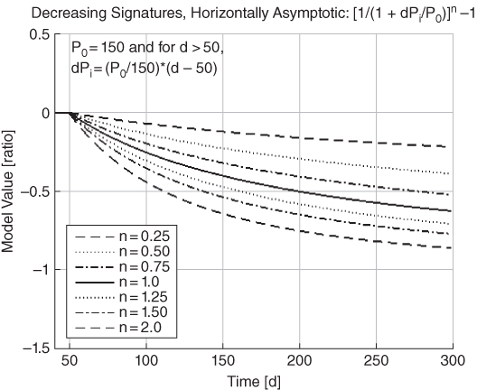
Figure 4.10 Power function #6: decreasing curves, horizontally asymptotic.
This is the mirror image of Eq. (4.13) with respect to the horizontal axis. As the magnitude of this type of signature becomes increasingly horizontal, changes in magnitude of noise begin to dominate changes in signal magnitude caused by degradation. The level of degradation for which functional failure is defined should be at or below the level where an incremental change in signal magnitude between samples equals the maximum magnitude of noise.
Power Function #7: Increasing Signatures, Slightly Curvilinear, Decreasing or Increasing Slope Angles
The following model is for a power function that produces characteristic signatures that increase, are slightly curvilinear, and have either a decreasing angle (see Figure 4.11) or an increasing angle (see Figure 4.12) depending on the value of the power n:
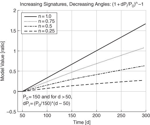
Figure 4.11 Power function #7: increasing curves, slightly curvilinear, decreasing slope angles.

Figure 4.12 Power function #7: increasing curves, slightly curvilinear, increasing slope angles.
At first glance, the signatures shown in the plots might appear to be straight lines; however, except for n = 1 (a straight‐line curve), the signatures are slightly curvilinear.
Power Function #8: Decreasing Signatures, Slightly Curvilinear, Decreasing or Increasing Slope Angles
The following model is for a power function that produces characteristic signatures that decrease, are slightly curvilinear; and have either a decreasing (see Figure 4.13) or increasing (see Figure 4.14) slope angle depending on the value of the power n:

Figure 4.13 Power function #8: decreasing curves, slightly curvilinear, decreasing slope angles.

Figure 4.14 Power function #8: decreasing curves, slightly curvilinear, increasing slope angles.
This is the mirror image of Eq. (4.15) with respect to the horizontal axis.
At first glance, the signatures might appear to be straight lines; however, except for n = 1 (a straight‐line curve), the signatures are slightly curvilinear.
Power Function #9: Increasing Signatures, Vertically or Horizontally Asymptotic
The following model is for a power function that produces characteristic signatures that increase and are vertically or horizontally asymptotic, depending on the value of the power n (see Figures 4.15 and 4.16):

Figure 4.15 Power function #9: increasing curves, vertically asymptotic, dPi < P0.

Figure 4.16 Power function #9: increasing curves, horizontally asymptotic, dPi < P0.
The model implies the following:
- When dPi < P0, the signatures are increasing for all values of n.
- As dPi → P0, the signatures become either vertically or horizontally asymptotic: the system approaches instability.
- When dPi > P0, the model is declared to be “not valid” and the system is defined as having ceased to function.
Power Function #10: Decreasing Signatures, Vertically or Horizontally Asymptotic
The following model is for a power function that produces characteristic signatures that decrease and are vertically or horizontally asymptotic, depending on the value of the power n (see Figures 4.17 and 4.18):

Figure 4.17 Power function #10: decreasing curves, vertically asymptotic, dPi < P0.

Figure 4.18 Power function #10: decreasing curves, horizontally asymptotic, dPi < P0.
This is the mirror image of Eq. (4.17) with respect to the horizontal axis. The model implies the following:
- When dPi < P0, the signatures are decreasing for all values of n.
- As dPi → P0, the signatures become either vertically or horizontally asymptotic: the system approaches instability.
- When dPi > P0, the model is declared to be “not valid” and the system is defined as having ceased to function.
Exponential Function #11: Increasing Signatures, Approximately Vertically Asymptotic
The following is a model of an exponential function that produces characteristic signatures that increase and become increasingly vertically asymptotic (see Figure 4.19):

Figure 4.19 Exponential function #11: increasing curves, vertically asymptotic.
As degradation increases, the signatures become approximately vertically asymptotic at dPi ≥ 5P0. It is recommended that functional failure be defined to occur when or before degradation reaches a value of dPi = 2P0.
Exponential Function #12: Decreasing Signatures, Approximately Vertically Asymptotic
The following is a model of an exponential function that produces characteristic signatures that decrease and become increasingly vertically asymptotic slopes (see Figure 4.20):

Figure 4.20 Exponential function #12: decreasing curves, vertically asymptotic.
This is the mirror image of Eq. (4.19) with respect to the horizontal axis. As degradation increases, the signatures become approximately vertically asymptotic at dPi ≥ 5P0. It is recommended that functional failure be defined to occur when or before degradation reaches a value of dPi = 2P0.
Exponential Function #13: Increasing Signatures, Horizontally Asymptotic
The following is a model of an exponential function that produces characteristic signatures that increase and become increasingly horizontally asymptotic (see Figure 4.21):

Figure 4.21 Exponential function #13: increasing curves, horizontally asymptotic.
As degradation increases, the signatures become horizontally asymptotic at dPi ≥ 5P0. It is recommended that functional failure be defined to occur when or before degradation reaches a value of dPi = 2P0.
Exponential Function #14: Decreasing Signatures, Horizontally Asymptotic
The following is a model of an exponential function that produces characteristic signatures that decrease and become increasingly horizontally asymptotic (see Figure 4.22):

Figure 4.22 Exponential function #14: decreasing curves, horizontally asymptotic.
This is the mirror image of Eq. (4.21) with respect to the horizontal axis. As degradation increases, the signatures become horizontally asymptotic at dPi ≥ 5P0. It is recommended that functional failure be defined to occur when or before degradation reaches a value of dPi = 2P0.
4.3.2 Example Plots of Representative FFP Degradation Signatures
Figures 4.3 – 4.22 present example plots of FFP signatures in response to increasing degradation.
4.3.3 Converting Decreasing Signatures to Increasing Signatures
The following degradation‐signature models produce decreasing signatures:
| Power function #2, Eq. (4.10): | f(dPi, P0) = − (dPi/P0)n |
| Power function #4, Eq. (4.12): | f(dPi, P0) = 1 − [1/(1 − dPi/P0)]n |
| Power function #6, Eq. (4.14): | f(dPi, P0) = [1/(1 + dPi/P0)]n − 1 |
| Power function #8, Eq. (4.16): | f(dPi, P0) = 1 − (1 + dPi/P0)n |
| Power function #10, Eq. (4.18): | f(dPi, P0) = (1 − dPi/P0)n − 1 |
| Exponential‐function #12, Eq. (4.20): | f(dPi, P0) = 1 − exp(dPi/P0) |
| Exponential‐function #14, Eq. (4.22): | f(dPi, P0) = exp(−dPi/P0) − 1 |
To reduce the number of models, transform decreasing signatures into increasing signatures by doing the following:
Using the method of Example 4.2, you can convert all of the decreasing signatures to increasing signatures. Then you get the results shown in Table 4.1.
Table 4.1 List of decreasing signatures and models and corresponding increasing models.
| Signature name | Decreasing model | Increasing model |
| Power function #2 | −(dPi/P0)n | (dPi/P0)n |
| Power function #4 | 1 − [1/(1 − dPi/P0)]n | [1/(1 − dPi/P0)]n − 1 |
| Power function #6 | [1/(1 + dPi/P0)]n − 1 | 1 − [1/(1 + dPi/P0)]n |
| Power function #8 | 1 − (1 + dPi/P0)n | (1 + dPi/P0)n − 1 |
| Power function #10 | (1 − dPi/P0)n − 1 | 1 − (1 − dPi/P0)n |
| Exponential function #12 | 1 − exp(dPi/P0) | exp(dPi/P0) − 1 |
| Exponential function #14 | exp(−dPi/P0) − 1 | 1 − exp(−dPi/P0) |
4.4 DPS Modeling: FFP to DPS Transform Models
In this section, we develop the models to transform FFP signature data into DPS data. To do that, we start with Eq. ( 4.4 ) and solve Eq. ( 4.5 ):
A solution set {dPi/P0} is a set of DPS data, {DPSi}, that is a degradation‐progression signature.
4.4.1 Developing Transform Models: FFP to DPS
We shall substitute FFP into Eq. (4.24), solve the result to get Eq. (4.25), and verify the solution. Verification shall consist of (i) producing FFP example data, (ii) performing a visual verification of the signature, (iii) transforming the example data to produce a DPS‐based signature, and (iv) performing a visual verification that the DPS‐based signature is an ideal transfer curve: a straight line.

Figure 4.23 Simulated FFP signatures: power function #1.

Figure 4.24 Simulated DPS from FFP signatures: power function #1.
Transform Model for Power Function #1
From Eq. ( 4.9 ), for the degradation‐signal model for power function #1, and from Eq. ( 4.24 ):
Since
we have
Figure 4.23 shows plots of simulated FFP signatures, and Figure 4.24 shows plots of DPS data after transforming the FFP signatures: the modeling for transform Eq. (4.26) is verified.
Transform Model for Power Function #3
From Eq. ( 4.11 ), the degradation‐signal model for power function #3, and from Eq. ( 4.24 ):
So
and therefore
Finally
Figure 4.25 shows plots of simulated FFP signatures, and Figure 4.26 shows plots of DPS data after transforming the FFP signatures: the modeling for transform Eq. (4.27) is verified.

Figure 4.25 Simulated FFP signatures: power function #3.

Figure 4.26 Simulated DPS from FFP signatures: power function #3.
Transform Model for Power Function #5
From Eq. ( 4.13 ), the degradation‐signal model for power function #5, and from Eq. ( 4.24 ):
So
and therefore
Finally,
Figure 4.27 shows plots of simulated FFP signatures, and Figure 4.28 shows plots of DPS data after transforming the FFP signatures: the modeling for transform Eq. (4.28) is verified.

Figure 4.27 Simulated FFP signatures: power function #5.

Figure 4.28 Simulated DPS from FFP signatures: power function #5.
Transform Model for Power Function #7
From Eq. ( 4.15 ), the degradation‐signal model for power function #7, and from Eq. ( 4.24 ):
So
and therefore
Figure 4.29 shows plots of simulated FFP signatures, and Figure 4.30 shows plots of DPS data after transforming the FFP signatures: the modeling for transform Eq. (4.29) is verified.

Figure 4.29 Simulated FFP signatures: power function #7.

Figure 4.30 Simulated DPS from FFP signatures: power function #7.
Transform Model for Power Function #9
From Eq. ( 4.17 ), the degradation‐signal model for power function #9, and from Eq. ( 4.24 ):
So
and
Figure 4.31 shows plots of simulated FFP signatures, and Figure 4.32 shows plots of DPS data after transforming the FFP signatures: the modeling for transform Eq. (4.30) is verified.

Figure 4.31 Simulated FFP signatures: power function #9.

Figure 4.32 Simulated DPS from FFP signatures: power function #9.
Transform Model for Exponential Function #11
From Eq. ( 4.19 ), the degradation‐signal model for exponential function #11, and from Eq. ( 4.24 )
so
and
Figure 4.33 shows plots of simulated FFP signatures, and Figure 4.34 shows plots of DPS data after transforming the FFP signatures: the modeling for transform Eq. (4.31) is verified.

Figure 4.33 Simulated FFP signatures: exponential function #11.

Figure 4.34 Simulated DPS from FFP signatures: exponential function #11.

Figure 4.35 Simulated FFP signatures: exponential function #13.

Figure 4.36 Simulated DPS from FFP signatures: exponential function #13.
Transform Model for Exponential Function #13
From Eq. ( 4.21 ), the degradation‐signal model for exponential function #13, and from Eq. ( 4.24 ):
So
and therefore
Finally,
Figure 4.35 shows plots of simulated FFP signatures, and Figure 4.36 shows plots of DPS data after transforming the FFP signatures: the modeling for transform Eq. (4.32) is verified.
4.4.2 Example Plots of FFP Signatures and DPS Signatures
Figures 4.23 – 4.36 present example plots of increasing FFP degradation signatures and their transforms to DPS.
4.5 FFS Modeling: Failure Level and Signature Modeling
Before you can transform a DPS into an FFS, you need to define and specify a threshold value of DPS data for functional failure. While it is possible to choose any such value, a better way is to define a threshold value of FFP signature data and then transform that value into a DPSBASED value. An example of why using an FFPBASED value is preferred is the following: it is always the case that if the value of a component is reduced to 0, the component has failed; similarly, if the value of a component has doubled in size, it would be reasonable to declare that component as failed. A qualitative assessment such as this is better made for FFPBASED values. As a matter of practice and preference, this book recommends that functional failure be defined when or before the value of a degrading component is reduced by or increased by 70%, which is when or before an FFPi value of 0.70.
4.5.1 Developing DPS‐Based Failure Level (FL) Models Using FFP Defined Failure Levels
For each of the representative sets of example FFP signatures, we shall use Eqs. ( 4.4 )–( 4.6 ) to solve Eq. (4.7) to create FLDPS models, which shall be verified by plotting and comparing FFP and DFP signatures using values for FLFFP and FLDPS:
and
DPS‐Based FL Model for Power Function #1
From Eq. ( 4.26 ), to transform an FFP signature for power function #1, and from Eq. ( 4.7 ):
So
DPS‐Based FL Model for Power Function #3
From Eq. ( 4.27 ), to transform an FFP signature for power function #3, and from Eq. ( 4.7 ):
DPS‐Based FL Model for Power Function #5
From Eq. ( 4.28 ), to transform an FFP signature for power function #5, and from Eq. ( 4.7 ):
DPS‐Based FL Model for Power Function #7
From Eq. ( 4.29 ), to transform an FFP signature for power function #7, and from Eq. ( 4.7 ):
DPS‐Based FL Model for Power Function #9
From Eq. ( 4.30 ), to transform an FFP signature for power function #9, and from Eq. ( 4.7 ):
DPS‐Based FL Model for Exponential Function #11
From Eq. ( 4.31 ), to transform an FFP signature for exponential function #11, and from Eq. ( 4.7 ):
DPS‐Based FL Model for Exponential Function #13
From Eq. ( 4.32 ), to transform an FFP signature for exponential function #11, and from Eq. ( 4.7 ):
4.5.2 Modeling Results for Failure Levels: FFP‐Based and DPS‐Based
The results of specifying an FFP‐based failure level (FLFFP) and converting that value to a DPS‐based failure level (FLDPS) should result in the two signatures reaching the threshold level for functional failure at the same point in time. The plots in Figures 4.37 – 4.43 confirm the expected results for various degradation signatures for various levels of functional failure.
4.5.3 Transforming DPS Data into FFS Data
There is a final signature transform we need to perform: from DPS data to FFS data. Using DPS data as input to a prediction system would cause that system to acquire knowledge about the value of DPS data at which functional failure occurs. We transform DPS data into DPS‐based FFS data using Eq. (3.18):
The advantage of this transform is the presence of a single model for all failure levels, which greatly simplifies prediction‐algorithm processing to produce prognostic information based on which a prognosis of system health can be made. We provide two examples as illustrations.
4.6 Heuristic‐Based Approach to Modeling of Signatures: Summary
This chapter presented a rationale for transforming CBD signatures into other signatures: FFP, DPS, and FFS. You learned that both an FFP and a DPS can be transformed into an FFS. You saw that an FFP is a normalized version of a CBD and that an FFP greatly reduces the number of signature models; and we showed that transforming an FFP into an FFS produces a very amenable signature to use as input for prediction algorithms.
The heuristic‐based approach to modeling signatures presented in this chapter is summarized as follows:
- Transform CBD signatures into FFP signatures.
- Transform FFP signatures into DPS data.
- Transform DPS data into FFS data.
The last transform requires the specification of an FFP‐based threshold level at which functional failure occurs, followed by the calculation of a DPS‐based threshold level of failure: this threshold value is used to transform DPS data into FFS data.
It is possible to use knowledge and analysis based on, for example, PoF and FMEA to derive an accurate DPS‐based model as a function of a change in system, an assembly, or a component parameter that is degrading: f(dPi, P0). In practice, however, highly accurate models are not required unless the system, the data sensor, and the data‐conditioning and transform‐processing routines produce noiseless data: data that is absolutely flat in the absence of degradation, data that varies with 100% correlation to degradation, and degradation that causes data to increase or decrease monotonically as degradation progresses.
This chapter described how, given a set of DPS models, you can transform CBD‐based data into an FFS that is amenable to processing by prediction algorithms to produce prognostic information. The objective is to produce prognostic information having an accuracy consistent with the signal‐to‐noise ratio (SNR) of that CBD‐based data; the sampling rate used to acquire that CBD‐based data; and the measurement accuracy of the system, especially the sensor and data converters (digital‐to‐analog and analog‐to‐digital) used to process and transform data.
Table 4.2 lists increasing FFP functions and the model, FFP‐to‐DPS transform, and FL(FFP) to FL(DPS) model. Not shown in the table is the DPS‐to‐FFS transform:
Table 4.2 Models: decreasing signature, increasing signature, FFP‐to‐DPS, and FL(FFP) to FL(DPS).
| Increasing signature function | FFP signature model | FFP‐to‐DPS transform model | FFP‐based FL to DPS‐based FL model |
| Power function #1 | (dPi/P0)n | (FFPi)1/n | ( FLFFP)1/n |
| Power function #3 | [1/(1 − dPi/P0)]n − 1 | 1 − 1/(FFPi + 1)1/n | 1 − 1/( FLFFP + 1)1/n |
| Power function #5 | 1 − [1/(1 + dPi/P0)]n | 1/(1 − FFPi)1/n − 1 | 1/(1 − FLFFP)1/n − 1 |
| Power function #7 | (1 + dPi/P0)n − 1 | (FFPi + 1)1/n − 1 | (FLFFP + 1)1/n − 1 |
| Power function #9 | 1 − (1 − dPi/P0)n | 1 − (1 − FFPi)1/n | 1 − (1 − FLFFP)1/n |
| Exp. function #11 | exp(dPi/P0) − 1 | ln(FFPi + 1) | ln(FLFFP + 1) |
| Exp. function #13 | 1 − exp(−dPi/P0) | ln(1/(1 − FFPi)) | ln(1/(1 − FLFFP)) |
In the next chapter, you will learn that signatures are not ideal: they contain, for example, offset errors, distortion, and noise – including signal variations due to feedback effects, multiple failure‐mode effects, and so on. Included in the next chapter are methods for mitigating and/or ameliorating such non‐ideality.
References
- Carr, J.J. and Brown, J.M. (2000). Introduction to Biomedical Equipment Technology, 4e. Upper Saddle River, NJ: Prentice Hall.
- Erickson, R. (1999). Fundamentals of Power Electronics. Norwell, MA: Kluwer Academic Publishers.
- Hofmeister, J., Goodman, D., and Wagoner, R. (2016). Advanced anomaly detection method for condition monitoring of complex equipment and systems. 2016 Machine Failure Prevention Technology, Dayton, Ohio, US, 24–26 May.
- Hofmeister, J., Wagoner, R., and Goodman, D. (2013). Prognostic health management (PHM) of electrical systems using conditioned‐based data for anomaly and prognostic reasoning. Chemical Engineering Transactions 33: 992–996.
- Hofmeister, J., Szidarovszky, F., and Goodman, D. (2017). An approach to processing condition‐based data for use in prognostic algorithms. 2017 Machine Failure Prevention Technology, Virginia Beach, Virginia, US, 15–18 May.
- Judkins, J.B. and Hofmeister, J.P. (2007). Non‐invasive prognostication of switch mode power supplies with feedback loop having gain, IEEE Aerospace Conference 2007, Big Sky, Montana, US, 4–9 Mar.
- Judkins, J.B., Hofmeister, J., and Vohnout, S. (2007). A prognostic sensor for voltage regulated switch‐mode power supplies. IEEE Aerospace Conference 2007, Big Sky, Montana, US, 4–9 Mar, Track 11–0804, 1–8.
- Kwon, D., Azarian, M.H., and Pecht, M. (2010). Degradation of Digital Signal Characteristics Due to Intermediate Stages of Interconnect Failure, 281–296. College Park, MD: Center for Adv. Life Cycle Eng. (CALCE), Univ. of Maryland.
- Texas Instruments. (1995). Understanding data converters. Application Report SLAA013.
- Viswanadham, P. and Singh, P. (1998). Failure Modes and Mechanisms in Electronic Packages, Chapter 7, 283–307. New York, NY: Chapman and Hall.
Further Reading
- Filliben, J. and Heckert, A. (2003). Probability distributions. In: Engineering Statistics Handbook. National Institute of Standards and Technology. http://www.itl.nist.gov/div898/handbook/eda/section3/eda36.htm.
- Tobias, P. (2003a). Extreme value distributions. In: Engineering Statistics Handbook. National Institute of Standards and Technology. https://www.itl.nist.gov/div898/handbook/apr/section1/apr163.htm.
- Tobias, P. (2003b). How do you project reliability at use conditions? In: Engineering Statistics Handbook. National Institute of Standards and Technology. https://www.itl.nist.gov/div898/handbook/apr/section4/apr43.htm.