Chapter 10
Analysis in ℝ
m
10.1 Derivatives
In this section, we review some of the key results in the differential calculus of one or more real variables. For the most part, proofs are not provided.
Let U be an open set in ℝ m , let F : U → ℝ n be a map, and let p be a point in U. We say that F is differentiable at p if there is a linear map L p : ℝ m → ℝ n such that

It can be shown that if such a map exists, it is unique. We call this map the differential of F at p and henceforth denote it by
In the literature, the differential of F at p is also called the derivative of F at p or the total derivative of F at p, and is denoted variously by dF p , dF p , DF(p), D p (F), or F'(p). We have chosen to include parentheses in the notation d p (F) to set the stage for viewing d p as a type of map.
It is usual to characterize d p (F) as being a “linear approximation” to F in the vicinity of p. For a more geometric interpretation, let us define the graph of F by
We can think of d p (F)(ℝ m ), which is a vector space, as being the “tangent space” to graph(F) at F(p). This is a generalization of the tangent line and tangent plane familiar from the differential calculus of one or two real variables.
We say that F is differentiable (on U) if it is differentiable at every p in U. To illustrate the difference between continuity and differentiability, consider the function f : ℝ → ℝ given by f(x) = |x|. As was observed in Section 9.4, f is continuous; however, it is not differentiable because there are two candidates for “tangent line” at x = 0.
We now specialize to the case n =1 and consider differentiable functions, turning our attention to differentiable maps below. Let f : U → ℝ be a function, and let p be a point in U. Consistent with (10.1.1), the differential of f at p is denoted by
We need to establish notation for coordinates on ℝ m . This notation will serve for the present chapter, but will need to be revised later on.
In this chapter, coordinates on ℝ m are denoted by (x 1 ,…,x m ) or ( y 1 ,…, y m ).
Let U be an open set in ℝ m , let f : U → ℝ be a function, and let p = (p 1,…,p m ) be a point in U. The partial derivative of f with respect to x i at p is defined by
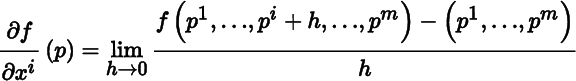
for i = 1,…,m, provided the limit exists. It is sometimes convenient to denote
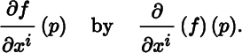
When m = 1, we denote

In this notation, the linear function d p (f) : ℝ → ℝ is given by

for all x in ℝ. More generally, we have the following result.
Thus, d p (f)(v) is nothing other than the directional derivative of f at p in the direction v, familiar from the differential calculus of two or more real variables.
Let U be an open set in ℝ m , let f : U → ℝ be a function, and suppose (∂f/∂x i )(p) exists for all p in U for i = 1,…,m. The partial derivative of f with respect to x i is the function

defined by the assignment
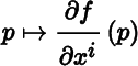
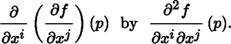
for all p in U. Now suppose (∂/∂x i )(∂f/∂x j )(p) exists for all p in U for i, j = 1,…,m. The second order partial derivative of f with respect to x i and x j is the function

defined by the assignment

for all p in U for i, j = 1,…,m, where we denote
Iterating in an obvious way, higher‐order partial derivatives of f are obtained. For k ≥ 2, a kth‐order partial derivative of f is denoted by

where the integers 1 ≤ i 1,i 2,…,i k ≤ m are not necessarily distinct.
Let us denote by C 0(U) the set of functions f : U → ℝ that are continuous on U. For k ≥ 1, we define C k (U) to be the set of functions f : U → ℝ such that all partial derivatives of f of order ≤ k exist and are continuous on U.
From Theorem 10.1.1, Theorem 10.1.2, and Theorem 10.1.4, we obtain the following result, which summarizes the relationship of continuity to differentiability for a function on an open set in ℝ m .
Let U be an open set in ℝ m , and let f : U → ℝ be a function. We say that f is (Euclidean) smooth (on U ) if f is in C k (U) for all k ≥ 0. The set of smooth functions on U is denoted by C ∞(U). In view of Theorem 10.1.5, C ∞(U) is the set of functions f on U with partial derivatives of all orders on U. It is sometimes said that smooth functions are “infinitely differentiable”.
We make C ∞(U) into both a vector space and a ring by defining operations as follows: for all functions f, g in C ∞(U) and all real numbers c, let

and
for all p in U. The identity element of the ring is the constant function 1 U that sends all points in U to the real number 1.
We now turn our attention to differentiable maps.
The next result is one of the workhorses of analysis and will be called upon frequently.
A remark on the above notation is in order. Instead of G ∘ F , it would be more precise, although somewhat cluttered, to write G| F(U) ∘ F . When there is a possibility of confusion or if it improves exposition, notation will be modified in this way.
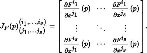
Let U be an open set in ℝ m , let F = (F 1,…, F n ) : U → ℝ n be a differentiable map, and let p be a point in U. The Jacobean matrix of F at p is the n × m matrix defined by

Denoting by ε and ℱ the standard bases for ℝ m and ℝ n , respectively, we have from (2.2.3), Theorem 10.1.2, and Theorem 10.1.8(b) that
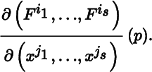
When m = n, the determinant det (J F (p)) is called the Jacobean determinant of F at p. Let 1 ≤ i 1 <…< i s ≤ m and 1 ≤ j 1 <…< j s ≤ n be integers, where 1 ≤ s ≤ min(m, n). Using multi‐index notation, the sub matrix of J F (p) consisting of the intersection of rows i 1,…,i s and columns j 1,…, j s (in that order) is
In the literature, the above matrix is commonly denoted by
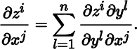
To give (10.1.4) a more traditional appearance, we continue with the above notation, let (z 1,…, z k ) be standard coordinates on ℝ k , and replace
with
Then (10.1.4) can be expressed as
Let U be an open set in ℝ m , and let F = (F 1,…,F n ) : U → ℝ n be a map. We say that F is smooth (on U) if the function F i is smooth for i = 1,…,m. Smooth maps will be our focus for the rest of the book.
The next result, which says that smoothness is ultimately a local phenomenon, will be used frequently, but usually without attribution.
A (parameterized) curve in ℝ m is a map λ : I → ℝ m , where I is an interval in ℝ that is either open, closed, half‐open, or half‐closed, and where the possibility that I is infinite is not excluded. Our focus will be on the case where I is a finite open interval, usually denoted by (a, b). Rather than provide a separate statement identifying the independent variable for the curve, most often denoted by t, and sometimes by u, it is convenient to incorporate this into the notation for λ, as in λ (t) : (a, b) → ℝ3. Let λ = (λ 1,…, λ m ). By definition, A is smooth [on (a, b)] if and only if λi is smooth for i = 1,…, m.
Suppose λ is in fact smooth. The (Euclidean) velocity of λ and the (Euclidean) acceleration of λ are the smooth curves
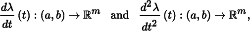
respectively; that is,

and

for all t in (a, b).
The next result is the key to later discussions about “vectors” and “tangent spaces”.
Not all maps of interest have domains that are open sets. For this reason we need an “extended” definition of smoothness to handle maps defined on sets that are not necessarily open. Let S be an arbitrary subset of ℝ
m
, and let F : S → ℝ
n
be a map. We say that F is (extended) smooth (on S) if for every point p in S, there is a neighborhood 풰 of p in ℝ
m
and a (Euclidean) smooth map ![]() such that F and
such that F and ![]() agree on S ⋂ 풰; that is,
agree on S ⋂ 풰; that is,![]() . Although in the preceding definition both 풰 and
. Although in the preceding definition both 풰 and ![]() might very well depend on p, the next result shows that this dependence can be avoided.
might very well depend on p, the next result shows that this dependence can be avoided.
For example, a curve λ(t) : [a, b] → ℝ
m
is smooth if and only if there is an interval ![]() containing [a, b] and a smooth curve
containing [a, b] and a smooth curve ![]() such that
such that ![]() .
.
10.2 Immersions and Diffeomorphisms
Let U be an open set in ℝ m , let F : U → ℝ n be a smooth map, where m ≤ n, and let p be a point in U. Since F is smooth on U, hence differentiable at p, we have from remarks in Section 10.1 that d p (F)(ℝ m ) can be viewed as the “tangent space” to the graph of F at F (p). We say that F is an immersion at p if the differential map d p (F) : ℝ m → ℝ n is injective, and that F is an immersion (on U) if it is an immersion at every p in U.
The next result gives alternative ways of characterizing an immersion.
Let U be an open set in ℝ m , let F, G : U → ℝ m be smooth maps, and let p be a point in U, where we note that both the domain and co domain of F and G are subsets of ℝ m . We say that F : U → F(U) is a diffeomorphism, and that U and F(U) are diffeomorphic, if F(U) is open in ℝ m , F : U → F(U) is injective, and F ‐1 : F(U) → ℝ m is smooth. We say that G is a local diffeomorphism at p if there is a neighborhood U' ⊆ U of p in ℝ m and a neighborhood V of G(p) in ℝ m such that G| U' : U' → V is a diffeomorphism. Then G is said to be a local diffeomorphism (on U) if it is a local diffeomorphism at every p in U. Evidently, every diffeomorphism is a local diffeomorphism.
It is straightforward to give “extended” versions of the preceding definitions using the extended definition of smoothness presented in Section 10.1.
The inverse map theorem (also called the inverse function theorem) underscores the close relationship between “smoothness” and “tangent space”. It is one of the most important results in analysis and will be called upon repeatedly.
10.3 Euclidean Derivative and Vector Fields
Let U be an open set in ℝ m , and let X : U → ℝ m be a map, where we note that both the domain and co domain of X are subsets of ℝ m . In the present context, we refer to X as a vector field (on U). To highlight the appearance of vector fields and to distinguish them from other types of maps, let us denote
for all p in U. We say that X vanishes at p if X p = (0,…,0), is no vanishing at p if X p ≠ (0,…,0), and is nowhere‐vanishing (on U) if it is no vanishing at every p in U.
Let us denote the set of smooth vector fields on U by ![]() (U). We make
(U). We make ![]() (U) into both a vector space over ℝ and a module over C
∞(U) by defining operations as follows: for all vector fields X, Y in
(U) into both a vector space over ℝ and a module over C
∞(U) by defining operations as follows: for all vector fields X, Y in ![]() (U), all functions f in C
∞(U), and all real numbers c, let
(U), all functions f in C
∞(U), and all real numbers c, let
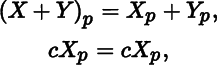
and
for all p in U. Let
where α i , β j are functions in C ∞(U) for i, j = 1,…, m. Then
and
The α
i are called the components of X. Let E
i
be the (constant) vector field in ![]() (U) defined by
(U) defined by
where 1 is in the ith position and 0s are elsewhere for i = 1,…, m.
The Euclidean derivative with respect to X consists of two maps, both denoted by D X . The first is
defined by
for all functions f in C ∞(U) and all p in U. The second is
defined by
for all vector fields Y in ![]() (U) and all p in U. It follows from Theorem 10.1.14(a) that (10.3.2) and (10.3.3) can be expressed as
(U) and all p in U. It follows from Theorem 10.1.14(a) that (10.3.2) and (10.3.3) can be expressed as

and
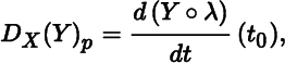
respectively, where λ(t) : (a, b) → U is any smooth curve such λ(t 0) = p and (dλ/dt)(t 0) = X p for some t 0 in (a, b). The existence of such a smooth curve is guaranteed by Theorem 10.1.13.
Evidently, the Euclidean derivatives of f and Y with respect to X evaluated at p have the same mathematical content as the differentials at p of f and Y evaluated at X p . Their difference, such as it is, amounts to a change of notation that emphasizes the role of X in the Euclidean derivative.
For vector fields X, Y in ![]() (U), we define a function
(U), we define a function
in C ∞(U) by the assignment
for all p in U.
The Euclidean derivative with respect to X satisfies fundamental algebraic properties, versions of which will reappear later in several settings.
Let U be an open set in ℝ
m
, and let X, Y be vector fields in ![]() (U). The second order Euclidean derivative with respect to X and Y
consists of two maps, both denoted by
(U). The second order Euclidean derivative with respect to X and Y
consists of two maps, both denoted by![]() . The first is
. The first is
defined by
for all functions f in C ∞(U). The second is
defined by
for all vector fields Z in ![]() (U).
(U).
10.4 Lie Bracket
Let U be an open set in ℝ m . Lie bracket is the map
defined by
for all vector fields X, Y in ![]() (U). We refer to [X, Y] as the Lie bracket of X and Y
.
(U). We refer to [X, Y] as the Lie bracket of X and Y
.
10.5 Integrals
Having discussed derivatives in Sections 10.1–10.4, we now briefly turn our attention to integrals.
Let [a i , b i ] be a closed interval in ℝ, where a i ≤ b i for i = 1,…,m. The set
is called a closed cell in ℝ m . The content of C is defined by
We observe that cont(C) = 0 if and only if a
i
= b
i
for some 1 ≤ i ≤ m. When m = 1, 2, 3, “content” is referred to as “length”, “area”, “volume”, respectively. To illustrate, consider the subset [0, 1] of ℝ and the “geometrically equivalent” subset [0,1] × [0, 0] of ℝ2. Then [0, 1] has a length of 1, while [0,1] × [0, 0] has an area of 0. A subset S of ℝm is said to have content zero if for every real number ε > 0, there is a finite collection {C
i
: 1 = 1,…,k} of closed cells such that ![]() and
and ![]() For example, [0, 1] × [0, 0] has content zero.
For example, [0, 1] × [0, 0] has content zero.
Let C be a closed cell in ℝ
m
, and let f : C → ℝ be a bounded function. We say that a finite collection {C
i
: 1 = 1,…,k} of closed cells in ℝ
m
is a partition of
C if each C
i
is a subset of C, the C
i
intersect only along their boundaries, and ![]() . For example, {[0, 1] × [0, 1], [1, 2] × [0, 1]} is a partition of [0, 2] × [0, 1]. Given a point p
i
in C
i
for i = 1,…,k, the sum Σ
I
f(p
i
) cont (C
i
) is an approximation to what we intuitively think of as the “content under the graph of f”. For each choice of partition of C and each choice of the pi, we get a corresponding sum. Using an approach analogous to that adopted in the integral calculus of one real variable, where inscribed and super scribed rectangles are used to approximate the area under the graph of a real‐valued function of one real variable, we define lower and upper integrals of f over C, denoted by
. For example, {[0, 1] × [0, 1], [1, 2] × [0, 1]} is a partition of [0, 2] × [0, 1]. Given a point p
i
in C
i
for i = 1,…,k, the sum Σ
I
f(p
i
) cont (C
i
) is an approximation to what we intuitively think of as the “content under the graph of f”. For each choice of partition of C and each choice of the pi, we get a corresponding sum. Using an approach analogous to that adopted in the integral calculus of one real variable, where inscribed and super scribed rectangles are used to approximate the area under the graph of a real‐valued function of one real variable, we define lower and upper integrals of f over C, denoted by ![]() and
and ![]() , respectively, to be limits of the preceding approximating sums. It can be shown that since f is bounded, both
, respectively, to be limits of the preceding approximating sums. It can be shown that since f is bounded, both ![]() and
and ![]() are finite. We say that f is (Riemann) integrable if
are finite. We say that f is (Riemann) integrable if ![]() and
and ![]() are equal. In that case, their common value, called the (Riemann) integral of f over C
, is denoted by
are equal. In that case, their common value, called the (Riemann) integral of f over C
, is denoted by

We need to be able to integrate functions over sets less restrictive than closed cells. Let S be a bounded set in ℝ m , and let f : S → ℝ be a bounded function. Since S is bounded, there is a closed cell C containing S. Let us define a function f C : C → ℝ by
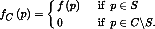
We say that f is (Riemann) integral if f C is integral. In that case, the (Riemann) integral of f over S is denoted by ∫ S f dx 1⋯dx m and defined by
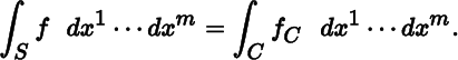
It can be shown that the inerrability of f and the value of ∫ S f dx 1⋯dx m are independent of the choice of closed cell containing S.
We now introduce a type of bounded set in ℝ m over which a certain type of function is always integrable. A subset D of ℝ m is called a domain of integration if it is bounded and its boundary in ℝ m has content zero. For example, a closed cell in ℝ m is a domain of integration.
Let U be an open set in ℝ m , and let f : U → ℝ be a continuous function that has compact support; that is, supp(f) is compact in U. By Theorem 9.2.2, U is the union of a collection of open balls in ℝ m . Using Theorem 9.1.5, it is easily shown that since supp(f ) is compact in U, it is contained in the union D of a finite sub collection of the open balls. Thus, supp(f ) ⊆ D ⊆ U. Furthermore, it can also be shown that D is a domain of integration. The
(Riemann) integral of f over U is denoted by ∫ U f dx 1⋯dx m and defined by
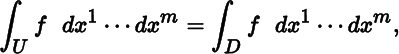
where the right‐hand side is given by (10.5.2). By Theorem 9.1.13, f is continuous on D, and by Theorem 9.1.22(b), f is bounded on supp(f), hence bounded on D. We have from Theorem 10.5.1 that the integral exists. It can be shown that the value of the integral is independent of the choice of domain of integration containing supp(f).
Let D be a domain of integration in ℝ m . It is clear that the function 1 D : D → ℝ with constant value 1 is continuous and bounded, so Theorem 10.5.1 applies. The content of D is defined by

It can be shown that when D is a closed cell in ℝ m , the definitions of cont(D) given by (10.5.1) and (10.5.4) agree.
10.6 Vector Calculus
In this section, we present a brief overview of the basic definitions and results of vector calculus. Much of what follows will be replaced later on with more modern counterparts expressed in the language of differential geometry.
Let U be an open set in ℝ3, let f, g be functions in C ∞(U), and let F = (F 1, F 2,F 3) : U → ℝ3 be a smooth map. The definitions of the classical differential operators in ℝ3 are given in Table 10.6.1, with the classical vector calculus notation shown alongside the notation to be used in this book. The use of “lap” for the Laplacian is not conventional, but it fits well with notation to be introduced later.
Table 10.6.1 Classical differential operators
| Operator | Definition |
| Gradient |

|
| Divergence |
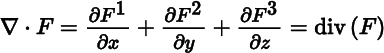
|
| Curl |

|
| Laplacian |
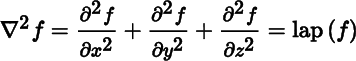
|
| Laplacian | ∇2 F = (lap(F 1), lap(F 2), lap(F 3)) = lap(F) |