Chapter 12
Curves and Regular Surfaces in 
Chapter 11 was devoted to a discussion of curves and regular surfaces in ℝ3 . A regular surface was defined to be a subset of ℝ3 with certain properties specified in terms of the subspace topology, smooth maps, immersions, homeomorphisms, and so on. The fact that ℝ3 has an inner product (which gives rise to a norm, which in turn gives rise to a distance function, which in turn gives rise to a topology) was relegated to the background—present but largely unacknowledged. The topological and metric aspects of ℝ3 were central to our discussion of what it means for a regular surface to be “smooth”, and in that way the inner product (through the distance function) was involved.
In this chapter, we continue our discussion of regular surfaces, but this time endow each tangent plane with additional linear structure induced by the linear structure on ℝ3
. Specifically, we view ℝ3
as either Euclidean 3‐space, that is, ![]() or Minkowski 3‐space, that is,
or Minkowski 3‐space, that is, ![]() and give each tangent plane the corresponding inner product or Lorentz scalar product obtained by restriction. It must be stressed that this additional linear structure changes nothing regarding the underlying regular surface. The definitions introduced in Chapter 11 remain in force, but we now express them somewhat differently. To that end, let us denote
and give each tangent plane the corresponding inner product or Lorentz scalar product obtained by restriction. It must be stressed that this additional linear structure changes nothing regarding the underlying regular surface. The definitions introduced in Chapter 11 remain in force, but we now express them somewhat differently. To that end, let us denote ![]() and
and ![]() collectively by
collectively by ![]() with the understanding that ν = 0 or 1 depending on the context. After introducing a series of definitions, we will speak of a regular surface as being a “regular surface in
with the understanding that ν = 0 or 1 depending on the context. After introducing a series of definitions, we will speak of a regular surface as being a “regular surface in ![]() ”. Again it must be emphasized that aside from the additional structure given to tangent planes, a regular surface in
”. Again it must be emphasized that aside from the additional structure given to tangent planes, a regular surface in ![]() is the same underlying regular surface considered in Chapter 11.
is the same underlying regular surface considered in Chapter 11.
12.1 Curves in 
Let ![]() be a smooth curve, and recall from Section 10.1 that the velocity of λ is the smooth curve
be a smooth curve, and recall from Section 10.1 that the velocity of λ is the smooth curve ![]() When V = 1, we say that λ is spacelike (resp., timelike, lightlike) if (dλ/dt)(t) is spacelike (resp., timelike, lightlike) for all t in (a, b). According to (4.1.1), the norm of (dλ/dt)(t) is
When V = 1, we say that λ is spacelike (resp., timelike, lightlike) if (dλ/dt)(t) is spacelike (resp., timelike, lightlike) for all t in (a, b). According to (4.1.1), the norm of (dλ/dt)(t) is

where we note the presence of (–1) v and the absolute value bars. The function ||dλ/dt|| : (a, b) → ℝ is called the speed of λ. Recall that λ is said to be regular if its velocity is nowhere‐vanishing. When ν = 0, this is equivalent to its speed being nowhere‐vanishing. We say that A has constant speed if there is a real number c such that ||(dλ/dt)(t)|| = (c) for all t in (a, b).
Let ![]() be an (extended) smooth curve. The length of λ (more precisely, the length of the image of λ) is defined by
be an (extended) smooth curve. The length of λ (more precisely, the length of the image of λ) is defined by

Other than their role in defining the above integral, we have little interest in the endpoints of [a, b]. In order to avoid having to consider one‐sided limits, we continue to frame the discussion in terms of ![]() but compute with
but compute with ![]() In short, we systematically confuse the distinction between [a, b] and (a, b).
In short, we systematically confuse the distinction between [a, b] and (a, b).
As the next result shows, the length of a smooth curve does not depend on the choice of parametrization.
12.2 Regular Surfaces in 
A regular surface is by definition a subset of ℝ3
. We now view a regular surface as a subset of ![]() , where V is left unspecified. The scalar product on
, where V is left unspecified. The scalar product on ![]() is given by
is given by
where ![]() and M are the Euclidean inner product and Minkowski scalar product, respectively.
and M are the Euclidean inner product and Minkowski scalar product, respectively.
Let M be a regular surface, and let p be a point in M. We obtain a symmetric tensor ![]() p
in
p
in ![]() by restricting the scalar product on
by restricting the scalar product on ![]() to
T
p
(M) × T
p
(M):
to
T
p
(M) × T
p
(M):
For brevity, we usually denote
Whether the notation 〈., .〉 refers to the scalar product on ![]() or the tensor
or the tensor ![]() will be clear from the context.
will be clear from the context.
The first fundamental form on
M is the map denoted by ![]() and defined by the assignment
and defined by the assignment ![]() for all p in M. In the literature,
for all p in M. In the literature, ![]() is often denoted by I. For vector fields X, Y in
is often denoted by I. For vector fields X, Y in ![]() (M), we define a function
(M), we define a function
in C ∞(M) by the assignment
for all p in M.
Since a subspace of an inner product space is itself an inner product space, when V = 0, ![]() p
is an inner product on T
p
(M) for all p in M. On the other hand, when V =1,
p
is an inner product on T
p
(M) for all p in M. On the other hand, when V =1, ![]() is bilinear and symmetric on T
p
(M), but there is no guarantee that it is nondegenerate. Furthermore, even if
is bilinear and symmetric on T
p
(M), but there is no guarantee that it is nondegenerate. Furthermore, even if ![]() is nondegenerate on each T
p
(M), it might be an inner product for some p and a Lorentz scalar product for others. In other words,
is nondegenerate on each T
p
(M), it might be an inner product for some p and a Lorentz scalar product for others. In other words, ![]() p
might not have the same index for all p in M. For these reasons, we make the following definition.
p
might not have the same index for all p in M. For these reasons, we make the following definition.
We say that ![]() is a metric (on
M) if:
is a metric (on
M) if:
[G1] ![]() p
is nondegenerate on T
p
(M) for all p in M.
p
is nondegenerate on T
p
(M) for all p in M.
[G2] ind (![]() p
) is independent of p in M.
p
) is independent of p in M.
When [G1] is satisfied, ![]() is a scalar product on T
p
(M) for all p in M. [G1] and [G2] are automatically satisfied when V = 0.
is a scalar product on T
p
(M) for all p in M. [G1] and [G2] are automatically satisfied when V = 0.
We say that a vector V in ![]() is normal at
p if V is in
T
p
(M)⊥
, where ⊥ is computed using the scalar product in
is normal at
p if V is in
T
p
(M)⊥
, where ⊥ is computed using the scalar product in ![]() . If V is also a unit vector, it is said to be unit normal at
p.
. If V is also a unit vector, it is said to be unit normal at
p.
Let V be a vector field along M. Recall that this means nothing more than V is a map from M to ![]() . Looked at another way, V is effectively a collection of vectors in
. Looked at another way, V is effectively a collection of vectors in ![]() , one for each p in M. Without further assumptions, there is no reason to expect V to be smooth; that is, V is not necessarily a vector field in
, one for each p in M. Without further assumptions, there is no reason to expect V to be smooth; that is, V is not necessarily a vector field in ![]() We say that V is a unit vector field if V
p
is a unit vector for all p in M, and that V is a normal vector field if V
p
is normal at p for all p in M. Clearly, a unit vector field is nowhere‐vanishing. When V is both a unit vector field and a normal vector field, it is said to be a unit normal vector field. For vector fields V, W along M, let us define the function
We say that V is a unit vector field if V
p
is a unit vector for all p in M, and that V is a normal vector field if V
p
is normal at p for all p in M. Clearly, a unit vector field is nowhere‐vanishing. When V is both a unit vector field and a normal vector field, it is said to be a unit normal vector field. For vector fields V, W along M, let us define the function
by the assignment
for all p in M. Let us also define the function
by the assignment
for all p in M. When ||V|| is nowhere‐vanishing, we define V/||V|| to be the vector field along M given by the assignment p → V p /‖V p ‖ for all p in M.
Here are two properties that a vector field V along M might satisfy:
[V1] T p (M)⊥ = ℝV p for all p in M.
[V2] 〈V p , W p 〉 is positive for all p in M, or negative for all p in M.
We observe that [V2] is equivalent to V p being either nonzero spacelike for all p in M, or timelike for all p in M.
We now show that properties [G1]–[G2] and [V1]–[V2] are closely related. For convenience of exposition, most of the results to follow are presented for arbitrary v. However, the findings for v = 0 are essentially trivial; it is the case v = 1 that is of primary interest.
Let M be a regular surface, and let ![]() be the first fundamental form on M. When
be the first fundamental form on M. When ![]() is a metric, the pair (M,
is a metric, the pair (M, ![]() ) is called a regular surface in
) is called a regular surface in
![]() In that case, we ascribe to
In that case, we ascribe to ![]() those properties of
those properties of ![]() that are independent of p. Accordingly,
that are independent of p. Accordingly, ![]() is said to be bilinear, symmetric, nondegenerate, and so on. The common value of the ind (
is said to be bilinear, symmetric, nondegenerate, and so on. The common value of the ind (![]() p
) is denoted by ind (
p
) is denoted by ind (![]() ) and called the index of
) and called the index of
![]() or the index of M.
or the index of M.
The next result shows that we could have defined a regular surface in ![]() using properties [V1] and [V2] instead of [G1] and [G2].
using properties [V1] and [V2] instead of [G1] and [G2].
Let
u
be an open set in ![]() , and let f be a function in
C
∞(U). The gradient of f
(in
, and let f be a function in
C
∞(U). The gradient of f
(in
![]() ) is the map
) is the map
defined by

for all p in U, where we note the presence of (–1) v . When v = 0, the above identity simplifies to (11.4.3), in which case, Grad (f) p = grad (f) p .
Let (M, g) be a regular surface in ![]() We have from Theorem 12.2.5 that there is a (not necessarily smooth) unit normal vector field V along M satisfying [V1] and [V2]. As pointed out in the proof of Theorem 12.2.4, since V is a unit vector field, [V2] is equivalent to: 〈V
p
, V
p
〉 = 1 for all p in M, or 〈V
p
, V
p
〉 = − 1 for all p in M. The common value of the 〈V
p
, V
p
〉 is denoted by ɛ
M
and called the sign of M
. Thus,
We have from Theorem 12.2.5 that there is a (not necessarily smooth) unit normal vector field V along M satisfying [V1] and [V2]. As pointed out in the proof of Theorem 12.2.4, since V is a unit vector field, [V2] is equivalent to: 〈V
p
, V
p
〉 = 1 for all p in M, or 〈V
p
, V
p
〉 = − 1 for all p in M. The common value of the 〈V
p
, V
p
〉 is denoted by ɛ
M
and called the sign of M
. Thus,
for all p in M. By Theorem 12.2.3(b), ɛ M is independent of the choice of unit normal vector field along M satisfying [V1] and [V2]. We have from Theorem 12.2.2(b) that
A convenient way to determine ind (![]() ) that avoids having to construct an orthonormal basis is to find ɛ
M
using (12.2.3) and then compute ind (
) that avoids having to construct an orthonormal basis is to find ɛ
M
using (12.2.3) and then compute ind (![]() ) using (12.2.4). The values of V, ind (
) using (12.2.4). The values of V, ind (![]() ), and ɛ
M
are related to each other as follows:
), and ɛ
M
are related to each other as follows:
| v |
ind ( |
ɛ M | (12.2.5) |
| 0 | 0 | 1 | |
| 1 | 1 | 1 | |
| 1 | 0 | –1 |
Continuing with the setup of Theorem 12.2.11, we note that the existence of a unit normal smooth vector field corresponding to each chart on M does not guarantee the existence of a unit normal smooth vector field along M. The reason is that the unit normal vector fields corresponding to different charts may not agree on the overlaps of images of their coordinate domains. In Section 12.7, we place additional structure on M that resolves this problem.
Let us now turn our attention to a special class of regular surfaces in![]() . Recall from Section 3.1 that the quadratic function q corresponding to
. Recall from Section 3.1 that the quadratic function q corresponding to ![]() is given by
is given by ![]() We consider three level sets of q, the first of which we have seen previously. For V = 0, the unit sphere is
We consider three level sets of q, the first of which we have seen previously. For V = 0, the unit sphere is
For v = 1, we define the pseudosphere by
and hyperbolic space by
Thus, ![]() is the set of (spacelike) unit vectors in
is the set of (spacelike) unit vectors in ![]() is the set of spacelike unit vectors in
is the set of spacelike unit vectors in ![]() and ℋ2
is the set of timelike unit vectors in
and ℋ2
is the set of timelike unit vectors in ![]() Taken together,
Taken together, ![]() ,
P
2, and ℋ2
are called the hyperquadrics in
,
P
2, and ℋ2
are called the hyperquadrics in ![]() and are denoted collectively by
and are denoted collectively by ![]() . We have the following table:
. We have the following table:
|
|
v | Type of vectors | (12.2.9) |
| S 2 | 0 | spacelike | |
| P 2 | 1 | spacelike | |
| H 2 | 1 | timelike |
It is interesting to observe that according to the table in part (d) of Theorem 12.2.12, the index of ℋ2
is 0. Thus, the tangent plane
T
p
(ℋ2) for each p in ℋ2
is an inner product space, despite the fact that
T
p
(ℋ2) is a subspace of the Lorentz vector space ![]()
We close this section with some definitions that will be used later on. Let (M, g) be a regular surface in ![]() let (U, φ) be a chart on M, and let ℋ = (H
1
, H
2) be the corresponding coordinate frame. We define functions
let (U, φ) be a chart on M, and let ℋ = (H
1
, H
2) be the corresponding coordinate frame. We define functions ![]() ij
in
C
∞(U) by
ij
in
C
∞(U) by
for all q in U for i, j = 1, 2. The matrix of ![]() with respect to ℋ is denoted by
with respect to ℋ is denoted by ![]() and defined by
and defined by
for all q in
U
. Setting p = φ (q), we recall from Section 3.1 that the matrix of ![]() with respect to ℋ
q
is
with respect to ℋ
q
is ![]() Thus, as a matter of notation,
Thus, as a matter of notation,
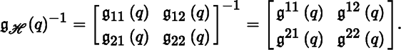
The inverse matrix of
![]() with respect to ℋ is denoted by
with respect to ℋ is denoted by ![]() and defined by
and defined by
for all q in U. It is usual to express the entries of ![]() with superscripts:
with superscripts:
The assignment ![]() defines functions
defines functions ![]() ij
in
C
∞(U) for i, j = 1, 2. Since [
ij
in
C
∞(U) for i, j = 1, 2. Since [![]() ij
] and [
ij
] and [![]() ij
] are symmetric matrices, the functions
ij
] are symmetric matrices, the functions ![]() ij
and
ij
and ![]() ij
are symmetric in i, j.
ij
are symmetric in i, j.
12.3 Induced Euclidean Derivative in
Let M be a regular surface, and let X be a vector field in ![]() . The
induced Euclidean derivative with respect to X
consists of two maps, both denoted by D
X
. The first is
. The
induced Euclidean derivative with respect to X
consists of two maps, both denoted by D
X
. The first is
defined by
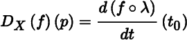
for all functions f in C ∞(M) and all p in M. The second is
defined by
for all vector fields V in ![]() and all p in M. (It will be clear from the context when the notation D
X
denotes the induced Euclidean derivative with respect to X as opposed to the Euclidean derivative with respect to X discussed in Section 10.3.)
and all p in M. (It will be clear from the context when the notation D
X
denotes the induced Euclidean derivative with respect to X as opposed to the Euclidean derivative with respect to X discussed in Section 10.3.)
We have from (11.5.1) and (11.7.1) that D X (f)(p) and D X (V) p can be expressed as
and

where λ(t) : (a, b) → M is any smooth curve such λ(t 0) = p and (dλ/dt)(t 0) = X p . Let V = (α 1, α 2, α 3). It follows from Theorem 11.7.2 and (12.3.2) that D X (V) p can also be expressed as
Following (12.2.2), for vector fields V, W in ![]() we define a function
we define a function
in C ∞(M) by the assignment
for all p in M.
The next result is a counterpart of Theorem 10.3.1.
By definition, if V is a vector field in ![]() then
D
X
(V) is a vector field in
then
D
X
(V) is a vector field in ![]() In particular, if Y is a vector field in
In particular, if Y is a vector field in ![]() then
D
X
(Y) is a vector field in
then
D
X
(Y) is a vector field in ![]() However, as the following example shows,
D
X
(Y) might not be a vector field in
However, as the following example shows,
D
X
(Y) might not be a vector field in![]() In other words, even though Y
p
is a vector in T
p
(M) for all p in M, the same might not be true of
D
X
(Y)
p
.
In other words, even though Y
p
is a vector in T
p
(M) for all p in M, the same might not be true of
D
X
(Y)
p
.
Let (M, ![]() ) be a regular surface in, let (U, φ) be a chart on M, and let ℋ = (H
1, H
2) and G be the corresponding coordinate frame and coordinate unit normal vector field. In keeping with earlier notation for a vector‐valued map, we denote
) be a regular surface in, let (U, φ) be a chart on M, and let ℋ = (H
1, H
2) and G be the corresponding coordinate frame and coordinate unit normal vector field. In keeping with earlier notation for a vector‐valued map, we denote
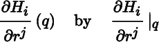
for all q in U for i, j = 1, 2. It follows from Theorem 8.4.10(b) and Theorem 12.2.11 that (G
q
, H
1|
q
, H
2|
q
) is a basis for ![]() Then (∂H
i
/∂r
j
) can be expressed as
Then (∂H
i
/∂r
j
) can be expressed as

where the ![]() called the Christoffel symbols, and the
ϑ
ij
are uniquely determined functions on U for i, j, k =1, 2.
called the Christoffel symbols, and the
ϑ
ij
are uniquely determined functions on U for i, j, k =1, 2.
We will make frequent use of the symmetry of the Christoffel symbols given by Theorem 12.3.3(d), usually without attribution. A quantity is said to be intrinsic to the geometry of a regular surface in ![]() if its definition depends only on the metric. Accordingly, Theorem 12.3.3(b) demonstrates that the Christoffel symbols are intrinsic.
if its definition depends only on the metric. Accordingly, Theorem 12.3.3(b) demonstrates that the Christoffel symbols are intrinsic.
We will see later that the Christoffel symbols are closely related to the “curvature” of a regular surface in ![]() . In particular, when all Christoffel symbols have constant value 0, the surface is “flat”. For example, consider Pln, the xy‐plane in
. In particular, when all Christoffel symbols have constant value 0, the surface is “flat”. For example, consider Pln, the xy‐plane in ![]() discussed in Section 13.1. Since
discussed in Section 13.1. Since ![]() it follows from Theorem 12.3.3(b) that each
it follows from Theorem 12.3.3(b) that each ![]() Thus, not surprisingly, Pln is “flat”.
Thus, not surprisingly, Pln is “flat”.
Let (M, ![]() ) be a regular surface in
) be a regular surface in![]() , and let X be a (not necessarily smooth) vector field on M. Let (U, φ) be a chart on M, and let (H
1, H
2) be the corresponding coordinate frame. Then
X ∘ φ
can be expressed as
, and let X be a (not necessarily smooth) vector field on M. Let (U, φ) be a chart on M, and let (H
1, H
2) be the corresponding coordinate frame. Then
X ∘ φ
can be expressed as

where the α i are uniquely determined functions on U, called the components of X with respect to (U, φ). The right‐hand side of (12.3.8) is said to express X in local coordinates with respect to (U, φ). Let us introduce the notation

for i, j = 1, 2.
12.4 Covariant Derivative on Regular Surfaces in 
Let (M, ![]() ) be a regular surface in
) be a regular surface in![]() , and let X, Y be vector fields in
, and let X, Y be vector fields in ![]() . As remarked in conjunction with Example 12.3.2, although the vector field
D
X
(Y) is in
. As remarked in conjunction with Example 12.3.2, although the vector field
D
X
(Y) is in ![]() it may not be in
it may not be in ![]() . In other words, even though Y
p
is a vector in T
p
(M) for all p in M, the same might not be true of
D
X
(Y)
p
. We need a definition of “derivative” that sends vector fields in
. In other words, even though Y
p
is a vector in T
p
(M) for all p in M, the same might not be true of
D
X
(Y)
p
. We need a definition of “derivative” that sends vector fields in ![]() to vector fields in
to vector fields in ![]() , thereby avoiding this problem. Our approach is pragmatic: we modify the induced Euclidean derivative, discussed in Section 12.3, by eliminating the part that is not tangential to M.
, thereby avoiding this problem. Our approach is pragmatic: we modify the induced Euclidean derivative, discussed in Section 12.3, by eliminating the part that is not tangential to M.
For each point p in M, we have by definition that ![]() p
is nondegenerate on the subspace T
p
(M) of
p
is nondegenerate on the subspace T
p
(M) of ![]() . It follows from Theorem 4.1.3 that
. It follows from Theorem 4.1.3 that ![]() is the direct sum
is the direct sum ![]() .For brevity, let us denote the projection maps
.For brevity, let us denote the projection maps ![]() and
and ![]() by tan
p
and nor
p
, respectively, so that
by tan
p
and nor
p
, respectively, so that
The covariant derivative with respect to X consists of two maps, both denoted by ∇ X . The first is
defined by
for all functions f in C ∞(M) and all p in M. The second is
defined by
for all vector fields Y in ![]() and all p in M, where D
X
(Y)
p
is given by (12.3.2). Observe that in the definition of the covariant derivative, all vector fields reside in
and all p in M, where D
X
(Y)
p
is given by (12.3.2). Observe that in the definition of the covariant derivative, all vector fields reside in ![]() . This is in contrast to the definition in Section 12.3 of the induced Euclidean derivative where vector fields in
. This is in contrast to the definition in Section 12.3 of the induced Euclidean derivative where vector fields in ![]() also appear.
also appear.
For vector fields X, Y in ![]() , we define a function
, we define a function
in C ∞(M) by the assignment
for all p in M.
Here are the basic formulas for computing with covariant derivatives.
Let (M, ![]() ) be a regular surface in
) be a regular surface in ![]() , and let X, Y be vector fields in
, and let X, Y be vector fields in ![]() . The second order covariant derivative with respect to X and Y
consists of two maps, both denoted by
. The second order covariant derivative with respect to X and Y
consists of two maps, both denoted by ![]() . The first is
. The first is
defined by
for all functions f in C ∞(M). The second is
defined by
for all vector fields Z in ![]() . These definitions are counterparts of the Euclidean versions given in Section 10.3.
. These definitions are counterparts of the Euclidean versions given in Section 10.3.
It was remarked following Theorem 12.3.3 that the Christoffel symbols corresponding to Pln have constant value 0 and this is related to Pln being “flat”. We see from Theorem 12.4.3(b) that in the context of Pln, the order of vector fields is immaterial when computing the second order covariant derivative. This is reminiscent of the Euclidean situation in ℝ
m
[see (Theorem 10.3.4(b)]. The following example shows that for the sphere ![]() , order is important.
, order is important.
12.5 Covariant Derivative on Curves in
Let (M, ![]() ) be a regular surface in
) be a regular surface in ![]() , let
λ(t) : (a, b) → M
be a smooth curve, and let
, let
λ(t) : (a, b) → M
be a smooth curve, and let ![]() be a map. In the present context, we refer to J as a vector field along λ. The set of smooth vector fields along λ is denoted by
be a map. In the present context, we refer to J as a vector field along λ. The set of smooth vector fields along λ is denoted by ![]() . As an example, if V is a vector field in
. As an example, if V is a vector field in ![]() , then
V ∘ λ
is a vector field in
, then
V ∘ λ
is a vector field in ![]() . We say that J is a (tangent) vector field on λ if J(t) is in
T
λ(t)(M) for all t in (a, b). Let us denote the set of smooth vector fields on λ by
. We say that J is a (tangent) vector field on λ if J(t) is in
T
λ(t)(M) for all t in (a, b). Let us denote the set of smooth vector fields on λ by ![]() . For example, dλ/dt, the velocity of λ, is in
. For example, dλ/dt, the velocity of λ, is in ![]() . As another example, if X is a vector field in
. As another example, if X is a vector field in ![]() (M), then
X ∘ λ
is a vector field in
(M), then
X ∘ λ
is a vector field in ![]() .
.
For a vector field J in ![]() , we have by definition that J(t) is a vector in
T
λ(t)(M) for all t in (a, b). But this is not necessarily so for (dJ/dt)(t). In particular, although the velocity of λ is in
, we have by definition that J(t) is a vector in
T
λ(t)(M) for all t in (a, b). But this is not necessarily so for (dJ/dt)(t). In particular, although the velocity of λ is in ![]() , its (Euclidean) acceleration may not be. We need a definition of “derivative” that avoids this problem. Our response is similar to the approach taken in Section 12.4.
, its (Euclidean) acceleration may not be. We need a definition of “derivative” that avoids this problem. Our response is similar to the approach taken in Section 12.4.
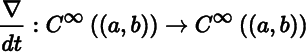
The covariant derivative on λ consists of two maps, both denoted by ∇/dt . The first is
defined by

for all functions f in C ∞((a, b)) and all t in (a, b). The second is
defined by

for all vector fields J in ![]() and all t in (a, b), where, following Section 12.4, tan
λ(t)
denotes the projection map
and all t in (a, b), where, following Section 12.4, tan
λ(t)
denotes the projection map ![]() .
.
The (covariant) acceleration of λ is defined to be the smooth curve

For vector fields J, K in ![]() , we define a function
, we define a function
in C ∞((a, b)) by the assignment
and all t in (a, b).
The definition of covariant derivative on a curve has an appealing physical interpretation. Imagine a “bug” that is confined to the 2‐dimensional world of a given regular surface in ![]() . For this creature, there is no “up” or “down”, only movements “on” the surface. Suppose the bug is scurrying along, tracing a smooth curve as it goes. From our vantage point in
. For this creature, there is no “up” or “down”, only movements “on” the surface. Suppose the bug is scurrying along, tracing a smooth curve as it goes. From our vantage point in ![]() , and knowing something about Newtonian physics, we determine that the bug has a certain velocity and nonzero (Euclidean) acceleration. For both us and the bug, velocity is entirely a tangential phenomenon. On the other hand, we observe the acceleration to have both tangential and normal components. But not so for the bug, which is oblivious to any such normal phenomena. This suggests that in order to quantify what we presume to be the acceleration felt by the bug, we should confine our attention to the tangential component. This is accomplished by taking the projection onto the tangent plane.
, and knowing something about Newtonian physics, we determine that the bug has a certain velocity and nonzero (Euclidean) acceleration. For both us and the bug, velocity is entirely a tangential phenomenon. On the other hand, we observe the acceleration to have both tangential and normal components. But not so for the bug, which is oblivious to any such normal phenomena. This suggests that in order to quantify what we presume to be the acceleration felt by the bug, we should confine our attention to the tangential component. This is accomplished by taking the projection onto the tangent plane.
Let (M, ![]() ) be a regular surface in
) be a regular surface in ![]() , let (U, φ) be a chart on M, and let (H
1, H
2) and G be the corresponding coordinate frame and coordinate unit normal vector field. Let
λ : (a, b) → M
be a smooth curve such that
λ((a, b)) ⊂ U
, and let J be a vector field in
, let (U, φ) be a chart on M, and let (H
1, H
2) and G be the corresponding coordinate frame and coordinate unit normal vector field. Let
λ : (a, b) → M
be a smooth curve such that
λ((a, b)) ⊂ U
, and let J be a vector field in ![]() . By Theorem 10.1.17 and Theorem 11.2.8, the map
. By Theorem 10.1.17 and Theorem 11.2.8, the map
is smooth. Then J(t) can be expressed as

where the α i are uniquely determined functions in C ∞(U), called the components of J with respect to (U, φ). The right‐hand side of (12.5.3) is said to express J in local coordinates with respect to (U, φ).
12.6 Lie Bracket in 
Let (M, ![]() ) be a regular surface in
) be a regular surface in ![]() . Lie bracket is the map
. Lie bracket is the map
defined by
for all vector fields X, Y in ![]() (M).
(M).
The next result shows that the Lie bracket on a regular surface in ![]() , formulated above in terms of the covariant derivative, can also be expressed in terms of the induced Euclidean derivative.
, formulated above in terms of the covariant derivative, can also be expressed in terms of the induced Euclidean derivative.
Here is a counterpart of Theorem 10.4.2.
12.7 Orientation in 
In Section 12.2, we defined a regular surface to be a regular surface in ![]() provided its first fundamental form satisfies certain properties. We then proceeded to demonstrate an equivalent formulation based on the existence of a particular type of unit normal vector field. Aside from an increase in geometric intuition, the latter approach offers computational advantages. For example, as remarked in connection with (12.2.4), it is usually more convenient to compute the index of a regular surface in
provided its first fundamental form satisfies certain properties. We then proceeded to demonstrate an equivalent formulation based on the existence of a particular type of unit normal vector field. Aside from an increase in geometric intuition, the latter approach offers computational advantages. For example, as remarked in connection with (12.2.4), it is usually more convenient to compute the index of a regular surface in ![]() indirectly using its sign. In this section, we explore orientation in the context of regular surfaces in
indirectly using its sign. In this section, we explore orientation in the context of regular surfaces in ![]() . The basic definition is given in terms of atlases, but once again unit normal vector fields play a prominent role. In what follows, we rely heavily on the discussion of orientation of vector spaces given in Section 8.2.
. The basic definition is given in terms of atlases, but once again unit normal vector fields play a prominent role. In what follows, we rely heavily on the discussion of orientation of vector spaces given in Section 8.2.
Let (M, ![]() ) be a regular surface in
) be a regular surface in ![]() , and let (U, φ) and
, and let (U, φ) and ![]() be overlapping charts on M. Let ℋ and
be overlapping charts on M. Let ℋ and ![]() be the corresponding coordinate frames, and let G and
be the corresponding coordinate frames, and let G and ![]() be the corresponding coordinate unit normal vector fields. Let
be the corresponding coordinate unit normal vector fields. Let ![]() , and let p be a point in W. Recall from Section 8.2 that the coordinate bases
, and let p be a point in W. Recall from Section 8.2 that the coordinate bases ![]() and
and ![]() are said to be consistent if
are said to be consistent if

We say that (U, φ) and ![]() are consistent if
are consistent if ![]() and
and ![]() are consistent for all p in W.
are consistent for all p in W.
Let (M, ![]() ) be a regular surface in
) be a regular surface in ![]() . An atlas for M is said to be consistent if every pair of overlapping charts in the atlas is consistent. We say that M is orientable if it has a consistent atlas. Suppose M is in fact orientable, and let
. An atlas for M is said to be consistent if every pair of overlapping charts in the atlas is consistent. We say that M is orientable if it has a consistent atlas. Suppose M is in fact orientable, and let ![]() be a consistent atlas for M. The triple (M,
be a consistent atlas for M. The triple (M, ![]() ,
, ![]() ) is called an oriented regular surface in
) is called an oriented regular surface in
![]() . Let p be a point in M, let (U, φ) be a chart in
. Let p be a point in M, let (U, φ) be a chart in ![]() at p, and let ℋ be the corresponding coordinate frame. Let
at p, and let ℋ be the corresponding coordinate frame. Let
where we recall from Section 8.2 that ![]() is the equivalence class of all bases for T
p
(M) (not just coordinate bases) that are consistent with
is the equivalence class of all bases for T
p
(M) (not just coordinate bases) that are consistent with ![]() . Let
. Let ![]() be another chart in
be another chart in ![]() at p, and let
at p, and let ![]() be the corresponding coordinate frame. Since
be the corresponding coordinate frame. Since ![]() is consistent, (U, φ) and
is consistent, (U, φ) and ![]() are consistent, hence
are consistent, hence  . This shows that the definition of
 ![]() (p) is independent of the choice of representative chart at p. We call the set of equivalence classes
(p) is independent of the choice of representative chart at p. We call the set of equivalence classes
the orientation induced by
![]() and say that M is oriented by
and say that M is oriented by
![]() . The notation (M,
. The notation (M, ![]() ,
, ![]() ), and sometimes (M,
), and sometimes (M, ![]() ,
, ![]() ,
, ![]() ), is used as an alternative to (M,
), is used as an alternative to (M, ![]() ,
, ![]() ).
).
Consider the map ι : ℝ2 → ℝ2 given by ι(r 1, r 2) = (−r 1, r 2). Since ι is a diffeomorphism and ι −1 = ι, (ι(U), φ ∘ ι) is a chart on M, where, for brevity, we denote ι| ι(U) by ι . Because
the corresponding coordinate frame and coordinate unit normal vector field are
and –G. It is easily shown using Theorem 11.3.3 that
is a consistent atlas for M. The orientation of M induced by –![]() is
is
where
We say that the orientation –![]() is the opposite of
is the opposite of
![]() .
.
Reviewing the proof of Theorem 12.2.12, we see that the preceding example rests on the gradient in question satisfying property [V2] of Section 12.2. More generally, we have the following extension of Theorem 12.2.10(b).
12.8 Gauss Curvature in
In this section, we describe a way of measuring the “curvature” of a regular surface in ![]() .
.
As part of the discussion of hyperquadrics ![]() in
in ![]() in Section 12.2, we observed that
in Section 12.2, we observed that ![]() is the set of (spacelike) unit vectors in
is the set of (spacelike) unit vectors in ![]() ,
, ![]() is the set of spacelike unit vectors in
is the set of spacelike unit vectors in ![]() , and ℋ2
is the set of timelike unit vectors in
, and ℋ2
is the set of timelike unit vectors in ![]() . In fact, more than just being sets, according to Theorem 12.2.12(a),
. In fact, more than just being sets, according to Theorem 12.2.12(a), ![]() is a regular surface in
is a regular surface in ![]() , and
, and ![]() and ℋ2
are regular surfaces in
and ℋ2
are regular surfaces in ![]() .
.
Let (M, ![]() ,
, ![]() ,
, ![]() ) be an oriented regular surface in
) be an oriented regular surface in ![]() , let
, let ![]() be the Gauss map, and let p be a point in M. Since
be the Gauss map, and let p be a point in M. Since ![]() is a unit normal vector at p, it follows from (12.2.3) that
is a unit normal vector at p, it follows from (12.2.3) that ![]() , where
, where ![]() is the quadratic function corresponding to
is the quadratic function corresponding to ![]() . Thus,
. Thus, ![]() is in the same hyperquadric for all p in M. Denoting the hyperquadric by
is in the same hyperquadric for all p in M. Denoting the hyperquadric by ![]() , we can now say that
, we can now say that ![]() is in
is in ![]() for all p in M. Thus,
for all p in M. Thus, ![]() can be expressed more precisely as
can be expressed more precisely as
The situation for ![]() is depicted in Figure 12.8.1, where
is depicted in Figure 12.8.1, where ![]() stands for
stands for ![]() for i = 1, 2, 3.
for i = 1, 2, 3.

Figure 12.8.1. Gauss map
The differential of ![]() at p is
at p is ![]() . By definition,
. By definition, ![]() is in
T
p
(M)⊥
. On the other hand, since
is in
T
p
(M)⊥
. On the other hand, since ![]() is in
is in ![]() , we have from Theorem 12.2.12(c) that
, we have from Theorem 12.2.12(c) that ![]() is also in
is also in ![]() . Since
T
p
(M)⊥
and
. Since
T
p
(M)⊥
and ![]() are both 1‐dimensional, it follows that
are both 1‐dimensional, it follows that ![]() , and then from Theorem 4.1.2(c) that
, and then from Theorem 4.1.2(c) that
We can therefore express the differential of ![]() at p as
at p as
Thus, ![]() is a linear map from
T
p
(M) to itself.
is a linear map from
T
p
(M) to itself.
For each point p in M, the Weingarten map at p is denoted by
and defined by
For all vectors v in T p (M), we have from (11.6.1) that

where λ(t) : (a, b) → M is any smooth curve such that λ(t 0) = p and (dλ/dt)(t 0) = v for some t 0 in (a, b). The Weingarten map is the linear map
defined by
for all vector fields X in ![]() and all p in M.
and all p in M.
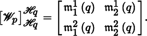
Let (U, φ) be a chart in ![]() , let ℋ = (H
1, H
2) be the corresponding coordinate frame, and let q be a point in U. The vector
, let ℋ = (H
1, H
2) be the corresponding coordinate frame, and let q be a point in U. The vector ![]() can be expressed as
can be expressed as
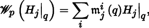
where the ![]() are uniquely determined functions in
C
∞(U). We then have from (2.2.2) and (2.2.3) that
are uniquely determined functions in
C
∞(U). We then have from (2.2.2) and (2.2.3) that
Let (M, ![]() ,
, ![]() ,
, ![]() ) be an oriented regular surface in
) be an oriented regular surface in ![]() , and let p be a point in M. Since
, and let p be a point in M. Since ![]() p
is bilinear and
p
is bilinear and ![]() is linear, we have the tensor
is linear, we have the tensor ![]() in
in ![]() defined by
defined by
for all vectors v, w in
T
p
(M). The second fundamental form on M
is the map denoted by ![]() and defined by the assignment
and defined by the assignment ![]() for all p in M. In the literature,
for all p in M. In the literature, ![]() is often denoted by II.
is often denoted by II.
For vector fields X, Y in ![]() , we define a function
, we define a function
in C ∞(M) by the assignment
for all p in M.
Let (U, φ) be a chart in ![]() , and let ℋ = (H
1, H
2) be the corresponding coordinate frame. We define functions
, and let ℋ = (H
1, H
2) be the corresponding coordinate frame. We define functions ![]() in
C
∞(U) by
in
C
∞(U) by
for all q in U for i, j = 1, 2, where p = φ(q). The matrix of
![]() with respect to ℋ is denoted by
with respect to ℋ is denoted by ![]() and defined by
and defined by

for all q in U.
Let (M, ![]() ,
, ![]() ,
, ![]() ) be an oriented regular surface in
) be an oriented regular surface in ![]() . The Gauss curvature is the smooth function
. The Gauss curvature is the smooth function
defined by
for all p in M. An intuitively appealing justification for this definition is provided below. For the moment, we simply observe that from (12.8.1), ![]() is defined in terms of
is defined in terms of ![]() , which is related to the “rate of change” of the unit normal vector field
, which is related to the “rate of change” of the unit normal vector field ![]() at p. In geometric terms, the greater the rate of change of
at p. In geometric terms, the greater the rate of change of ![]() , the greater the “curvature” we expect M to have at p.
, the greater the “curvature” we expect M to have at p.
It follows from Theorem 4.7.4 and Theorem 12.8.2(b) that ![]() has two (not necessarily distinct) real eigenvalues, which we denote by
κ
1(p) and
κ
2(p).
has two (not necessarily distinct) real eigenvalues, which we denote by
κ
1(p) and
κ
2(p).
The next result uses material on “local diffeomorphisms” from Section 14.6 and “area” from Section 19.10. It is included here because it provides a rationale for the definition of Gauss curvature when ν = 0.
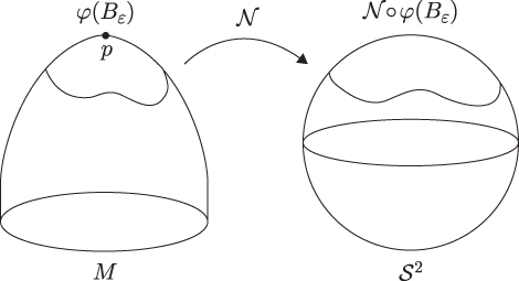
Figure 12.8.2. Diagram for Theorem 12.8.5
Figure 12.8.2 provides the geometric intuition for Theorem 12.8.5. Since M as depicted is highly curved at p, the area of ![]() is correspondingly greater than the area of
φ(B
ε
), leading to a larger value of
is correspondingly greater than the area of
φ(B
ε
), leading to a larger value of ![]() .
.
In ![]() , the plane, cylinder, and cone all have a constant Gauss curvature of 0. This is not surprising for the plane, but is perhaps counterintuitive for the cylinder and cone. The explanation is that the cylinder and cone can be obtained from (portions of) the plane by smooth deformations that involve bending but not stretching. This keeps the “intrinsic” geometry of the deformed plane intact, thereby preserving the Gauss curvature at each point. The sphere has constant positive Gauss curvature, while the traction, which is shaped like a bugle, has constant negative Gauss curvature. The Gauss curvature of the hyperboloid of one sheet (two sheets) is negative (positive) but no constant. The torus has a region where the Gauss curvature is positive, and one where it is negative, with a transition zone in between where the Gauss curvature is 0.
, the plane, cylinder, and cone all have a constant Gauss curvature of 0. This is not surprising for the plane, but is perhaps counterintuitive for the cylinder and cone. The explanation is that the cylinder and cone can be obtained from (portions of) the plane by smooth deformations that involve bending but not stretching. This keeps the “intrinsic” geometry of the deformed plane intact, thereby preserving the Gauss curvature at each point. The sphere has constant positive Gauss curvature, while the traction, which is shaped like a bugle, has constant negative Gauss curvature. The Gauss curvature of the hyperboloid of one sheet (two sheets) is negative (positive) but no constant. The torus has a region where the Gauss curvature is positive, and one where it is negative, with a transition zone in between where the Gauss curvature is 0.
| Section |
Geometric object in |
Gauss curvature |
| 13.1 | plane | 0 |
| 13.2 | cylinder | 0 |
| 13.2 | cone | 0 |
| 13.4 | sphere | 1/R 2 |
| 13.5 | tractoid | –1 |
| 13.6 | hyperboloid of one sheet | –1/(2x 2 + 2y 2 – 1)2 |
| 13.7 | hyperboloid of two sheets | 1/(2x 2 + 2y 2 + 1)2 |
| 13.8 | torus | cos(ϕ)/[cos(ϕ) + R] |
In ![]() , the pseudo sphere has constant positive Gauss curvature, while hyperbolic space has constant negative Gauss curvature. It is interesting to observe that the hyperboloid of one sheet and the pseudo sphere are defined in terms of the same underlying surface. The difference in their Gauss curvatures is due entirely to the fact that one resides in the inner product space
, the pseudo sphere has constant positive Gauss curvature, while hyperbolic space has constant negative Gauss curvature. It is interesting to observe that the hyperboloid of one sheet and the pseudo sphere are defined in terms of the same underlying surface. The difference in their Gauss curvatures is due entirely to the fact that one resides in the inner product space ![]() , and the other in the Lorentz vector space
, and the other in the Lorentz vector space ![]() . A similar remark applies to the hyperboloid of two sheets and hyperbolic space.
. A similar remark applies to the hyperboloid of two sheets and hyperbolic space.
| Section |
Geometric object in |
Gauss curvature |
| 13.9 | pseudo sphere | 1 |
| 13.10 | hyperbolic space | –1 |
12.9 Riemann Curvature Tensor in 
The Riemann curvature tensor for a regular surface (M, ![]() ) in
) in ![]() is the map
is the map
defined by
for all vector fields X, Y, Z in ![]() (M); that is,
(M); that is,
for all p in M. The large parentheses are included to make it clear that each of the four terms in the preceding identity is a vector field in ![]() (M) evaluated at the point p, and as such is a vector in T
p
(M
). Since (R(X, Y)Z)
p
is not a real number, using the term “tensor” to describe R is something of a misnomer. This conflict is resolved in Theorem 19.5.5. The expression R
p
(X
p
, Y
p
) Z
p
has no meaning—at least not yet.
(M) evaluated at the point p, and as such is a vector in T
p
(M
). Since (R(X, Y)Z)
p
is not a real number, using the term “tensor” to describe R is something of a misnomer. This conflict is resolved in Theorem 19.5.5. The expression R
p
(X
p
, Y
p
) Z
p
has no meaning—at least not yet.
We presented an instance in Example 12.4.4 where the second order covariant derivatives ![]() and
and ![]() are not equal. As the next result shows, the difference between these two vector fields is precisely R(X, Y)Z.
are not equal. As the next result shows, the difference between these two vector fields is precisely R(X, Y)Z.
For computational purposes, it is helpful to have a local coordinate expression for R.
We observed in Section 12.3 that the Christophe symbols are intrinsic. It follows from (12.9.2) and (12.9.3) that the same is true of the Riemann curvature tensor.
It is a remarkable feature of (12.9.2) that no partial derivatives of the component functions appear in the expression. This crucial observation underlies the next two results.
Let (M, g) be a regular surface in ![]() , and define a map
, and define a map
also called the Riemann curvature tensor, by
for all vector fields X, Y, Z, W in ![]() (M); that is,
(M); that is,
for all p in M. By definition, ℛ(X, Y, Z, W) is a function in C ∞(M). Since ℛ(X, Y, Z, W)(p) is a real number, calling ℛ a “tensor” is perhaps justified. We return to this issue below.
We noted in conjunction with (12.9.2) and (12.9.3) that the Riemann curvature tensor R is intrinsic. In view of (12.9.18), the same can be said of the Riemann curvature tensor ℛ. Just as was the case for (12.9.2), there are no partial derivatives of the component functions in (12.9.18). This observation underlies the next two results, which are counterparts of Theorem 12.9.4 and Theorem 12.9.5, and are proved similarly.
Let (M, ![]() ) be a regular surface in
) be a regular surface in ![]() , let p be a point in M, and let
v
be a vector in T
p
(M). According to Theorem 15.1.2, there is a vector field X in
, let p be a point in M, and let
v
be a vector in T
p
(M). According to Theorem 15.1.2, there is a vector field X in ![]() (M) such that X
p
= v. Taken in conjunction with Theorem 12.9.4, Theorem 12.9.5, Theorem 12.9.9, and Theorem 12.9.10, this allows us to give R and R interesting interpretations. We define a map
(M) such that X
p
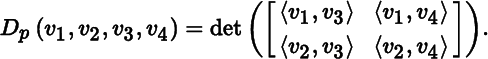
= v. Taken in conjunction with Theorem 12.9.4, Theorem 12.9.5, Theorem 12.9.9, and Theorem 12.9.10, this allows us to give R and R interesting interpretations. We define a map
by
and a map
by
for all vectors v
1,v
2,v
3,v
4 in T
p
(M), where X
1, X
2, X
3, X
4 are any vector fields in ![]() (M) such that
(M) such that
By Theorem 12.9.4 and Theorem 12.9.9, respectively, R p and ℛ p are independent of the choice of vector fields, so the definitions makes sense. It follows from (12.9.17) and the above identities that

By Theorem 12.9.10, ℛ
p
is in ![]() , and by Theorem 12.9.5, R
p
is in Mult (T
p
(M)3,T
p
(M)). This provides a justification for calling ℛ a “tensor”, and to a lesser extent a rationale for doing the same with R. Another tensor of interest in
, and by Theorem 12.9.5, R
p
is in Mult (T
p
(M)3,T
p
(M)). This provides a justification for calling ℛ a “tensor”, and to a lesser extent a rationale for doing the same with R. Another tensor of interest in ![]() is
is ![]() , as defined by (6.6.7):
, as defined by (6.6.7):
The name traditionally given to the next result is “Theorem Egregious”, which is Latin for “remarkable theorem”. The rationale for this impressive title is given below.
As remarked earlier, the Riemann curvature is intrinsic, whether we are dealing with R or ℛ. The Gauss curvature is defined using the Gauss map, which in turn is defined using the second fundamental form. For this reason, it would appear that the Gauss curvature depends on factors that are “external”. However, part (b) of the Theorem Egregious shows that the Gauss curvature is in fact intrinsic, something that is unexpected and indeed “remarkable”. The next result makes the same point using local coordinates.
12.10 Computations for Regular Surfaces in 
We showed in Theorem 11.4.2 and Theorem 11.4.3 that graphs of surfaces and surfaces of revolution are regular surfaces. In this section, we view them as regular surfaces in ![]() and develop specific formulas for computing the coordinate frame, Gauss map, first and second fundamental forms, Gauss curvature, and sign. For surfaces of revolution in
and develop specific formulas for computing the coordinate frame, Gauss map, first and second fundamental forms, Gauss curvature, and sign. For surfaces of revolution in ![]() , formulas for the Christophe symbols and eigenvalues are also provided.
, formulas for the Christophe symbols and eigenvalues are also provided.