14.1 Smooth Manifolds

Many of the definitions presented in this and subsequent chapters are adaptations of ones we encountered in the study of curves and surfaces.

Let M be a topological space. A chart on M is a pair (U,  φ), where U is an open set in M and φ : U → ℝ ^m is a map such that:

• [C1] φ(U) is an open set in ℝ ^m .
• [C2] φ : U → φ(U) is a homeomorphism.

We refer to U as the coordinate domain of the chart, to φ as its coordinate map, and to m as the dimension of the chart. For each point p in U , we say that (U,  φ) is a chart at p . (Note that in the definition of regular surfaces, coordinate maps went from open sets in ℝ² to open sets in the regular surface, whereas now traffic is in the opposite direction.) When U = M , we say that (M,  φ) is a covering chart on M , and that M is covered by (M,  φ). In the present context, the component functions of φ are denoted by φ = (x ¹,  …,  x ^m ) rather than φ = (φ ¹,  …,  φ ^m ), and are said to be local coordinates on U . This choice of notation is adopted specifically to encourage the informal identification of the point p in M with its local coordinate counterpart φ(p) = (x ¹(p), …,  x ^m (p)), in ℝ ^m We often denote

where (x ⁱ ) = (x ¹,  …,  x ^m ). The charts (U,  φ) and on M are said to be overlapping if is nonempty. In that case, the map

is called a transition map. For brevity, we usually denote

and in a similar manner often (but not always) drop the “restriction” subscript from other notation when the situation is clear from the context. An atlas for M is a collection of charts on M such that the U _α form an open cover of M ; that is, M = ∪ _α ∈ A U _α . At this point, there is no requirement that charts have the same dimension.

A topological m ‐manifold is a pair , where M is a topological space and is an atlas for M such that:

• [T1] Each chart in has dimension m .
• [T2] The topology of M has a countable basis.
• [T3] For every pair of distinct points p ₁,  p ₂ in M , there are disjoint open sets U ₁ and U ₂ in M such that p ₁ is in U ₁ and p ₂ is in U ₂ .

Observe that [T1] refers exclusively to the atlas , whereas [T2] and [T3] have to do with the topological structure of M . Properties [T2] and [T3] are technical requirements needed for certain constructions and will not be further elaborated upon.

Let be a topological m ‐manifold. We have from Theorem 14.1.2 that m is an invariant of , which we refer to as the dimension of M and denote by dim(M).

It can be shown that the connected components of a topological space are closed sets in the topological space. In the case of a topological manifold, the connected components have additional properties.

Let be a topological m ‐manifold, and let (U,  φ) and be overlapping charts on M . We say that (U,  φ) and are smoothly compatible if the transition maps and are (Euclidean) smooth. Since , this is equivalent to either or being a (Euclidean) diffeomorphism. We say that the atlas is smooth if any two overlapping charts in are smoothly compatible. A smooth atlas for M is also called a smooth structure on M . Recall that in our study of charts on regular surfaces, coordinate maps were assumed to be smooth, where smoothness was defined using relevant properties of the coordinate domain in ℝ² and the ambient space ℝ³ . Since M does not have such inherent properties, we have turned Theorem 11.2.9, a result on the smoothness of transition maps for regular surfaces, into a definition of smoothness for topological manifolds. We will see further examples of this approach as we proceed, where a theorem about “surfaces” becomes a definition for “manifolds”.

We say that a topological m ‐manifold is a smooth m ‐manifold if is a smooth atlas. It is often convenient to adopt the shorthand of referring to M as a smooth m ‐manifold, with understood from the context. Furthermore, when it is not important to specify the dimension of M , we refer to or simply M as a smooth manifold.

A smooth atlas for M is said to be maximal if it is not properly contained in any larger smooth atlas for M . This means that any chart on M that is smoothly compatible with every chart in is already in . It can be shown that every smooth atlas for M is contained in a unique maximal smooth atlas. A given topological space can have distinct smooth atlases that generate the same maximal smooth atlas. On the other hand, it is also possible for a topological space to have distinct smooth atlases that give rise to distinct maximal smooth atlases. Accordingly, we adopt the following convention.

Throughout, any chart on a smooth manifold comes from the underlying smooth atlas or its corresponding maximal atlas.

We noted in connection with Theorem 1.1.10 that all m‐dimensional vector spaces are isomorphic to ℝ ^m (viewed as a vector space). In light of Example 14.1.4, it should come as no surprise that any m ‐dimensional vector space has a smooth structure induced by ℝ ^m (now viewed as a smooth m ‐manifold).

Recall the discussion on product topologies in Theorem 9.1.6 and Theorem 9.1.12.

For example, it can be shown that the product manifold of m copies of ℝ is precisely ℝ ^m with the standard smooth structure.

14.2 Functions and Maps

Let M be a smooth manifold, and let f : M → ℝ be a function. Since M and ℝ are topological spaces, we know what it means for f to be continuous (on M ). Motivated by Theorem 11.5.1, we say that f is smooth (on M ) if for every point p in M , there is a chart (U,  φ) at p such that the function f ∘ φ ⁻¹ : φ(U) → ℝ is (Euclidean) smooth. The set of smooth functions on M is denoted by C ^∞(M). We make C ^∞(M) into both a vector space and a ring by defining operations as follows: for all functions f,  g in C ^∞(M) and all real numbers c , let

and

for all p in M .

The next result is reminiscent of Theorem 11.5.1.

We now turn our attention to maps. Let M and N be smooth manifolds, and let F : M → N be a map. Since M and N are topological spaces, we understand what is meant by F being continuous (on M ). With Theorem 11.6.1 as motivation, we say that F is smooth (on M ) if for every point p in M , there is a chart (U,  φ) at p and a chart (V,  ψ) at F(p) such that F(U) ⊆ V and the map ψ ∘ F ∘ φ ⁻¹ : φ(U) → ℝ ⁿ is (Euclidean) smooth. The condition F(U) ⊆ V is included as part of the definition of smoothness to ensure that the next result holds.

We close this section with a brief look at two important methods of construction on smooth manifolds—bump functions and partitions of unity.

A glance at Figure 14.2.2(b) explains why a function such as β is called a bump function. Bump functions are often called upon to extend the domain of a smooth map, as in the proof of the next result.

Although far from being intuitive, partitions of unity are indispensable for certain constructions in differential geometry, and we will see several such applications. The basic idea is to define the mathematical object of interest (for example, a function, vector field, or integral) on each set in the given open cover, and then form a weighted average using the π _α as weights to combine the individual contributions into a mathematical object defined on all of M . Because of part (c), there are no issues of convergence of infinite series.

14.3 Tangent Spaces

In the introduction to Part III, it was remarked that a crucial step in developing the theory of what we now call smooth manifolds is to devise a way of defining “tangent vector” when there is no ambient space. The definition created by differential geometers and provided here meets this challenge in an ingenious fashion. Framed in algebraic terms, it is both mathematically elegant and computationally convenient. However, it unfortunately lacks intuitive appeal compared to the methods adopted for surfaces, where tangent vectors were defined in terms of derivatives of smooth curves and could be thought of as “arrows”. Later on we will see that the algebraic approach leads to a theory closely resembling that developed for surfaces, thereby lending the algebraic theory a certain geometric flavor.

Before proceeding, we need to establish some notation. In Chapter 10, coordinates on ℝ ^m were denoted by (x ¹,  …,  x ^m ) or (y ¹,  …,  y ^m ). In Chapter 11 and Chapter 12, it was necessary to clearly distinguish between coordinates on ℝ² and ℝ³ . For ℝ² , the notation used was (r ¹,  r ²) or (r,  s), and for ℝ³ , it was (x ¹,  x ²,  x ³) or (x,  y,  z). In Chapter 13, coordinates on ℝ² and ℝ³ were denoted by (x,  y) and (x,  y,  z), respectively. The former choice was made because in the setting of graphs of functions, ℝ² was identified with the xy ‐plane in ℝ³ _. That brings us to the present chapter, and beyond.

Henceforth, coordinate maps will be denoted by ( x ¹ ,  …,   x ^m ) or ( y ¹ ,  …,   y ^m ) , except for standard coordinates on ℝ ^m , which will be denoted by ( r ¹ ,  …,   r ^m ) or ( s ¹ ,  …,   s ^m ) .

Let M be a smooth manifold, and let p be a point in M . A (tangent) vector at p is defined to be a linear function

that satisfies the following product rule:

(14.3.1)

for all functions f,  g in C ^∞(M). The set of tangent vectors at p is denoted by T _p (M) and called the tangent space of M at p . The zero vector in T _p (M), denoted by 0, is the tangent vector that sends all functions in C ^∞(M) to the real number 0. We make T _p (M) into a vector space by defining operations as follows: for all vectors v,  w in T _p (M) and all real numbers c , let

and

for all functions f in C ^∞(M).

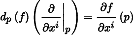
Let (U,  φ = (x ⁱ )) be a chart at p . The partial derivative with respect to x ⁱ at p is the map

defined by

(14.3.2)

for all functions f in C ^∞(M), where we denote

(14.3.3)

The right‐hand side of (14.3.2) is simply the ordinary (Euclidean) partial derivative of f ∘ φ ⁻¹ with respect to r ⁱ at φ(p). When m = 1, we denote

Note that although the x ⁱ have the domain U , the (∂/∂x ⁱ )| _p have the domain C ^∞(M), as opposed to C ^∞(U).

The next result is reminiscent of Theorem 11.4.1.

Throughout, any open set in a smooth m ‐manifold is viewed as a smooth m ‐manifold.

Theorem 14.3.2(a) and Theorem 14.3.3(b) show that tangent vectors operate locally.

Let V be an m ‐dimensional vector space that we suppose has the standard smooth structure, so that V is a smooth m ‐manifold. For each vector v in V , the tangent space T _v (V) is an m ‐dimensional vector space. In an obvious way, we identify T _v (V) with V (viewed as a vector space), and write

(14.3.4)

Let M be a smooth m ‐manifold, let p be a point in M , and let (U,  φ = (x ⁱ )) be a chart at p . The second order partial derivative with respect x ⁱ and x ^j at p is the map

defined by

for all functions f in C ^∞(M), where we denote

14.4 Differential of Maps

To define the differential map between two manifolds, we need a way to send vectors in one tangent space to vectors in another tangent space, and in a linear fashion. With the algebraic approach to vectors, this turns out to be surprisingly straightforward. Let M and N be smooth manifolds, let F : M → N be a smooth map, and let p be a point in M . For each vector v in T _p (M), define a map

by

(14.4.1)

for all functions g in C ^∞(N). Since g ∘ F is in C ^∞(M), the definition makes sense.

Continuing with above notation, the differential of F at p is the map

defined by the assignment

for all vectors v in T _p (M).

The remaining results of this section give the basic properties of differential maps.

The next result is a generalization of Theorem 14.3.5.

14.5 Differential of Functions

Let M be a smooth manifold, let f be a function in C ^∞(M), let p be a point in M , and let (U,  φ = (x ⁱ )) be a chart at p . Viewing ℝ as a smooth 1‐manifold, we have the differential map

(14.5.1)

A covering chart for ℝ is (ℝ,  id_ℝ = r), where r is the standard coordinate on ℝ. The corresponding coordinate basis at f(p) is ((d/dr)| _f(p)). Then Theorem 14.4.6(a) and id_ℝ = r give

(14.5.2)

Using (14.3.4), we identify T _f(p)(ℝ) with ℝ, and write T _f(p)(ℝ) = ℝ. To be consistent, we also identity the basis ((d/dr)| _f(p)) for T _f(p)(ℝ) with the basis (1) for ℝ. Then (14.5.1) and (14.5.2) become

(14.5.3)

and

(14.5.4)

for i = 1,  …,  m . Let us denote the dual space

The usual identification of a vector space with its double dual gives

With the next result, we recover an identity that is familiar from the differential calculus of several real variables, except that here “differentials” replace “infinitesimals”.

14.6 Immersions and Diffeomorphisms

In this brief section, we generalize the discussion of immersions and diffeomorphisms in Section 10.2 to the setting of smooth manifolds.

Let M and N be smooth manifolds, where dim(M) ≤ dim(N), let F : M → N be a smooth map, and let p be a point in M . We say that F is an immersion at p if the differential map d _p (F) : T _p (M) → T _F(p)(N) is injective, and that F is an immersion (on M ) if it is an immersion at every p in M .

Now suppose M and N have the same dimension, and let G,  H : M → N be smooth maps. We say that G is a diffeomorphism, and that M and N are diffeomorphic, if G is bijective and G ⁻¹ : N → M is smooth. We say that H is a local diffeomorphism at p if there is a neighborhood U of p in M and a neighborhood V of H(p) in N such that H| _U : U → V is a diffeomorphism. Then H is said to be a local diffeomorphism (on M ) if it is a local diffeomorphism at every p in M .

14.7 Curves

The following definitions are borrowed more or less directly from Section 10.1 and Section 11.1.

A (parametrized) curve on a smooth manifold M is a map λ : I → M , where I is an interval in ℝ that is either open, closed, half‐open, or half‐closed, and where the possibility that I is infinite is not excluded. Our focus will be on the case where I is a finite open interval, usually denoted by (a,  b). Rather than provide a separate statement identifying the independent variable for the curve, most often denoted by t , and sometimes by u , it is helpful to incorporate this into the notation for λ , as in λ(t) : I → M . When I is a closed interval [a,  b] and λ is continuous, we say that λ joins λ(a) to λ(b). It is convenient to adopt the following convention.

Henceforth, when required by the context, the interval I is assumed to contain 0 .

Consider the curve λ(t) : (a,  b) → M . Viewing (a,  b) as a smooth 1‐manifold, we say that λ is smooth [on ( a ,   b ) ] if it is smooth as a map between smooth manifolds. Suppose λ is in fact smooth. For a given point t in (a,  b), we have the differential map

A covering chart for (a,  b) is ((a,  b), id (a, b) = r), where r is the standard coordinate on (a,  b). The corresponding coordinate basis at t is ((d/dr)| _t ). It follows that

(14.7.1)

for all t in (a,  b). Thus, for all functions f in C ^∞((a,  b)),

(14.7.2)

In an effort to ensure that the notation adopted for smooth manifolds resembles as much as possible the notation from differential calculus, let us denote

(14.7.3)

We continue to indulge in the usual (and sometimes confusing) practice of obscuring the difference between a variable and its value. With this understanding, (14.7.1) and (14.7.2) become:

(14.7.4)

and

(14.7.5)

We refer to (dλ/dt)(t) as the velocity of λ at t .

It was remarked in the introduction to Part III that the algebraic approach to defining tangent vectors gives rise to results that have something of the geometric flavor found in the theory of surfaces. We close this section with several such instances.

Let M be a smooth manifold, let p be a point in M , and let v be a vector in T _p (M). We have from the preceding theorem that there is a smooth curve λ(t) : (a,  b) → M such that λ(t ₀) = p and (dλ/dt)(t ₀) = v for some t ₀ in (a,  b). Let X be a vector field in . Then X _p is a vector in T _p (M), hence there corresponds such a smooth curve. We will make use of these observations frequently.

14.8 Submanifolds

Having defined smooth manifolds, it is natural to consider subsets with corresponding properties. Let be a smooth ‐manifold, and let M be a subset of that is a smooth m ‐manifold in its own right. Without further assumptions, there is no reason to expect a connection between the topologies on and M , and likewise for their smooth structures. We say that M is an m ‐submanifold of if:

• [S1] M has the subspace topology.
• [S2] The inclusion map ι : is an immersion.

Suppose M is in fact an m‐submanifold of . It follows from [S2] that . We say that M is a hypersurface of if Since ι : is an immersion, for each point p in M , the differential map d _p (ι) : is injective. Given a vector v in T _p (M), the image vector d _p (ι)(v) behaves as follows: for all functions f in C ^∞(M),

We adopt the established convention of identifying T _p (M) with its image under d _p (ι). Thus, T _p (M) is viewed as a vector subspace of , and we write

(14.8.1)

Reflecting on the above definition of a submanifold, [S1] seems like an obvious requirement, but the same cannot be said of [S2]. Theorem 14.8.2 gives some insight into [S2], but its rationale is far from transparent. Rather than search for a deeper understanding of [S2], we change course and provide an alternative perspective on submanifolds.

For a given integer 1 ≤ k ≤ m , we define a type of projection map : ℝ ^m  → ℝ ^k  × {0} ^m − k by

Let U be an open set in ℝ ^m , and let S be a subset of U . We say that S is a k ‐slice of U if .

The above notation is rather cumbersome. Henceforth, x ⁱ | _M ∩ U will be abbreviated to x ⁱ for i = 1,  …,  m . In this revised notation, we denote

and

We require two further results on submanifolds, both of which are straightforward consequences of Theorem 14.8.3.

We saw in Theorem 14.3.3(a) that an open set in a smooth manifold is itself a smooth manifold. The next result says that it is also a submanifold.

Throughout, any open set in a smooth manifold is viewed as an open submanifold.

14.9 Parametrized Surfaces

A parametrized surface on a smooth manifold M is a smooth map of the form

where ε > 0 is a real number. For a given point r in (a,  b), we define a smooth curve

by

for all s in (−ε,  ε). Similarly, for a given point s in (−ε,  ε), we define a smooth curve

by

for all r in (a,  b). In keeping with the terminology introduced in the context of surfaces of revolution, we refer to σ _r as the latitude curve (or transverse curve) corresponding to r , and to σ _s as the longitude curve corresponding to s . In most applications, we tend to think of σ as a family of longitude curves indexed by s .

Let us now consider the smooth curve σ _s from the perspective of Section 14.7. For a given point s in (−ε,  ε), and using (14.7.3), we denote

(14.9.1)

According to (14.7.4),

We define (∂σ/∂s)(r,  s) similarly.