Looking back at the material presented on smooth manifolds and smooth manifolds with a connection, we see that many of the concepts and results motivated by our study of regular surfaces and regular surfaces in
have been recovered—but not all. Missing from our recent efforts has been any discussion of “length” and “area”. To address this shortfall, it is necessary to endow smooth manifolds with additional structure, which entails a consideration of semi‐Riemannian manifolds.
19.1 Semi‐Riemannian Manifolds
The following material builds on portions of the discussion in Section 12.2. Let M be a smooth m‐manifold, and let
be a symmetric tensor field in
, so that
is a symmetric tensor in
for all p in M. We say that
is a metric on M if:
[G1]
is nondegenerate on Tp(M) for all p in M.
[G2] ind
is independent of p in M.
When [G1] is satisfied,
is a scalar product on Tp(M) for all p in M; or equivalently, (Tp(M),
is a scalar product space for all p in M.
Suppose
is in fact a metric. In that case, the pair
is said to be a semi‐Riemannian m‐manifold. We ascribe to
those properties of
that are independent of p. Accordingly,
is said to be bilinear, symmetric, nondegenerate, and so on. The common value of the ind
is denoted by ν and called the index of
or the index of M. The common signature of the
is denoted by (ε1, …, εm) and called the signature of
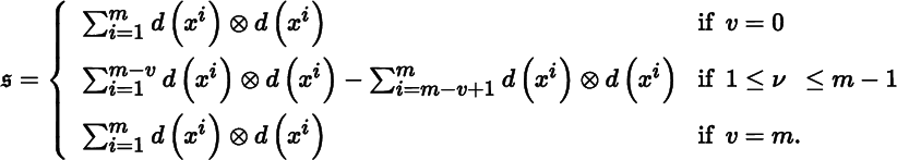
or the signature of M. For brevity, we usually denote
When ν = 0, we say that M is a Riemannian m‐manifold, and when m ≥ 2 and ν = 1, M is said to be a Lorentz m‐manifold. A semi‐Riemannian m‐manifold with a connection is a triple
, where
is a semi‐Riemannian m‐manifold and ∇ is a connection on M. For the time being, we do not assume that
and ∇ are related.
We have already encountered several semi‐Riemannian manifolds, although we were not in a position to use such terminology at the time. For example, semi‐Euclidean (m, ν)‐space
is a semi‐Riemannian m‐manifold of index ν. In particular, Euclidean m‐space
is a Riemannian m‐manifold, and Minkowski m‐space
is a Lorentz m‐manifold. With tensor notation now at our disposal, we can express
in local coordinates as
To our list of semi‐Riemannian manifolds, let us add the unit sphere
and hyperbolic space ℋ2, which are Riemannian 2‐manifolds, and the pseudosphere
, which is a Lorentz 2‐manifold. In fact, each of the regular surfaces in
described in Sections 13.1–13.8 is a Riemannian 2‐manifold. We now provide a less obvious example of a Riemannian 2‐manifold.
The remainder of this section presents definitions that will play a role later on.
Let
be a semi‐Riemannian m‐manifold, and let X, Y be vector fields in
. We say that X is a unit vector field if Xp is a unit vector for all p in M, and that X and Y are orthogonal vector fields if Xp and Yp are orthogonal for all p in M.
Let us define a function
in C∞(M) by the assignment
for all p in M. Similarly, for a smooth curve λ : (a, b) → M and vector fields J, K in
, we define a function
in C∞((a, b)) by the assignment
for all t in (a, b).
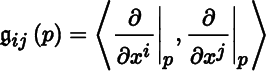
Let (U, (xi)) be a chart on M, and let
be the corresponding coordinate frame. We define functions
in C∞(U) by
(19.1.1)
for all p in U for i, j = 1, …, m. The matrix of
with respect to
is denoted by
and defined by
for all p in U. Recall from Section 3.1 that the matrix of
with respect to
is
. Thus, as a matter of notation,
The inverse matrix of
with respect to
is denoted by
and defined by
for all p in U. It is usual to express the entries of
with superscripts:
The assignment
defines functions
in C∞(U) for i, j = 1, …, m. Since
and
are symmetric matrices, the functions
and
are symmetric in i, j.
Let
be a semi‐Riemannian manifold, and let M be a submanifold of
. We say that
is a semi‐Riemannian submanifold of
if
is a metric on M. In that case, by definition: (i)
is nondegenerate on Tp(M) for all p in M, and (ii) ind
is independent of p in M. The common value of the ind
is denoted by ind
and called the index of
or the index of M. The common signature of the
is called the signature of
or the signature of M. We say that
is a Riemannian (Lorentz) submanifold if
, viewed as a semi‐Riemannian manifold in its own right, is a Riemannian (Lorentz) manifold. When
is a Riemannian (Lorentz) submanifold of
and also a hypersurface, we refer to
as a Riemannian (Lorentz) hypersurface of
. Observe that if
is a Riemannian manifold, then
is automatically a Riemannian submanifold. On the other hand, if
is a Lorentz manifold and
is a semi‐Riemannian submanifold, then the latter could be either a Riemannian or a Lorentz submanifold. To illustrate, we have from Theorem 12.2.12(d) and Theorem 14.8.2 that
is a Riemannian hypersurface of the Riemannian 3manifold
, while ℋ2 is a Riemannian hypersurface and
is a Lorentz hypersurface of the Lorentz 3‐manifold
.
Suppose
is a semi‐Riemannian hypersurface of
, and let p be a point in M. According to (14.8.1), Tp(M) can be viewed as a vector subspace of
. It follows from Theorem 4.1.3 that
, and then from Theorem 1.1.18 that Tp(M)⊥ is 1‐dimensional. We say that a vector v in
is normal at p if v is in Tp(M)⊥ If v is also a unit vector, it is said to be unit normal at p. In that case, since v is nonzero, we have Tp(M)⊥ = ℝv. Let V be a (not necessarily smooth) vector field along M. We say that V is a normal vector field if Vp is normal at p for all p in M. When V is both a unit vector field and a normal vector field, it is said to be a unit normal vector field.
Theorems 12.2.2–12.2.5 generalize in a straightforward fashion to the setting of a semi‐Riemannian hypersurface of a semi‐Riemannian manifold. It follows from the generalization of Theorem 12.2.5 that there is a (not necessarily smooth) unit normal vector field V along M such that 〈Vp, Vp〉 is independent of p in M. The common value of the 〈Vp, Vp〉 is denoted by ɛM and called the sign of M. Thus,
for all p in M. We have from the generalization of Theorem 12.2.2(b) that
19.2 Curves
Let
be a semi‐Riemannian manifold, let λ(t) : (a, b) → M be a smooth curve, and let g(u) : (c, d) → (a, b) be a diffeomorphism. The smooth curve λ ∘ g(u) : (c, d) → ℝ3 is said to be a smooth reparametrization of λ. Recall from Section 15.1 that the velocity of λ is the smooth curve (dλ/dt)(t) : (a, b) → M, and that λ is said to be regular if its velocity is nowhere‐vanishing. The speed of λ is the (not necessarily smooth) curve ∥(dλ/dt)(t)∥ : (a, b) → M. When ν = 0, λ is regular if and only if its speed is nowhere‐vanishing. We say that λ has constant speed if there is a real number c such that ∥(dλ/dt)(t) ∥ = c for all t in (a, b). It is said that λ is spacelike (resp., timelike, lightlike) if (dλ/dt)(t) is spacelike (resp., timelike, lightlike) for all t in (a, b). Also, λ is said to be future‐directed (past‐directed) if (dλ/dt)(t) is future‐directed (past‐directed) for all t in (a, b).
Let λ(t) : [a, b] → M be a smooth curve on a closed interval. The length of λ is defined by
(19.2.1)
19.3 Fundamental Theorem of Semi‐Riemannian Manifolds
Let
be a semi‐Riemannian manifold with a connection. Without further assumptions, there is no reason to expect
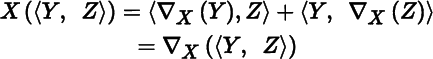
and ∇ to be related. We say that ∇is compatible with
if
(19.3.1)
for all vector fields X, Y, Z in
, where the second equality follows from (18.1.1). According to definitions given in Section 18.4,
is a tensor field in
, and
is parallel (with respect to∇) provided
.
The next result is sometimes called “the miracle of semi‐Riemannian geometry”
Throughout, unless stated otherwise, the connection on a semi‐Riemannian manifold is the Levi‐Civita connection.
With this convention, when we say that
is a semi‐Riemannian manifold, it is implicit that there is a connection on M, and it is the Levi‐Civita connection. On the other hand, the notation
indicates that
is a semi‐Riemannian manifold with a connection, but not necessarily the Levi‐Civita connection.
Christoffel symbols for a regular surface in
were introduced in Section 12.3, and for a smooth manifold with a connection in Section 18.2. As the next result shows, with a metric at our disposal, we can recover the identity for Christoffel symbols given in Theorem 12.3.3(b).
The next result shows that in normal coordinates at a given point, a semi‐Riemannian m‐manifold of index ν behaves like
with respect to the metric and the Christoffel symbols at that point.
Let
be a semi‐Riemannian manifold, let U be an open set in M, and let
be a frame on U. We say that
is orthonormal if
is an orthonormal basis for Tp(M) for all p in U. When M is oriented,
is said to be positively oriented if
is positively oriented for all p in U.
We call upon Theorem 19.3.7 often, but usually without attribution.
19.4 Flat Maps and Sharp Maps
In this section, we present manifold versions of the flat maps and sharp maps defined in Section 3.3, Section 6.2, and Section 6.3.
Let
be a semi‐Riemannian manifold. For a given vector field X in
, we define a map
by
(19.4.1)
for all vector fields Y in
.
The flat map on M is the map
defined by the assignment
for all vector fields X in
. Thus, as a matter of notation,
The sharp map
on M is defined to be the inverse of
; that is,
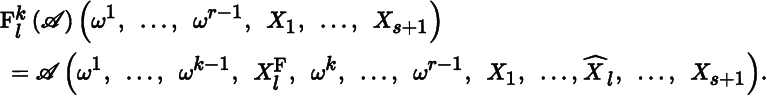
Let 1 ≤ k ≤ r and 1 ≤ l ≤ s + 1 be integers (so that r ≥ 1 and s ≥ 0). The (k, l)‐flat map is denoted by
and defined (using Theorem 15.7.2) for all tensor fields
in
, all covector fields ω1, …, ωr − 1 in
, and all vector fields X1, …, Xs + 1 in
as follows, where
indicates that an expression is omitted:
[F1] For r = 1 (so that k = 1):
[F2] For r ≥ 2 and 1 ≤ k ≤ r − 1:
[F3] For r ≥ 2 and k = r:
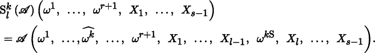
Similarly, let 1 ≤ k ≤ r + 1 and 1 ≤ l ≤ s be integers (so that r ≥ 0 and s ≥ 1). The (k, l)‐sharp map is denoted by
and defined (using Theorem 15.7.2) for all tensor fields
in
, all covector fields ω1, …, ωr + 1 in
, and all vector fields X1, …, Xs − 1 in
as follows:
[S1] For s = 1 (so that l = 1):
[S2] For s ≥ 2 and 1 ≤ l ≤ s − 1:
[S3] For s ≥ 2 and l = s:
19.5 Representation of Tensor Fields
The representation of tensor fields on smooth manifolds was considered in
Section 15.7
. Let us now return to this topic with the additional structure afforded by semi‐Riemannian manifolds. We introduce smooth manifold counterparts of the representation map and scalar product map presented in Section 5.3 and Section 6.4, respectively, and link them using the characterization map defined in Section 15.5 and
Section 15.7
. The notation is admittedly horrendous, but the ideas are essentially those introduced in the much less complicated setting of scalar product spaces.
Let
be a semi‐Riemannian manifold. Following Section B.5, we denote by
the C∞(M)‐module of C∞(M)‐multilinear maps from
to
, and by
the C∞(M)‐module of C∞(M)‐multilinear maps from
to C∞(M).
Let us define a map
called the scalar product map, by
for all maps Ψ in Mult
and all vector fields X1, …, Xs + 1 in
. We observe that
is the smooth manifold counterpart of the map defined by 6.4,1).
Let us now define a map
called the representation map, by
(19.5.1)
for all maps Ψ in
, all covector fields ω in
, and all vector fields X1, …, Xs in
. We observe that ℜs is the smooth manifold counterpart of the map defined by (5.3.1). When s = 1, we denote
and obtain
Then
(19.5.2)
for all maps Ψ in
, all covector fields ω in
, and all vector fields X in
.
Our efforts in this section, and much of what we previously developed in the area of “representations”, have ultimately been directed at obtaining the following result. It provides the long‐awaited justification for using the term “tensor” when referring to the torsion tensor and curvature tensor.
19.6 Contraction of Tensor Fields
The contraction of tensor fields on smooth manifolds was considered in Section 15.14. We now return to this topic armed with the properties of semi‐Riemannian manifolds.
Let
be a semi‐Riemannian manifold. Corresponding to the (k, 1)‐flat map
and the (k, l)‐sharp map
introduced in Section 19.4, we now define manifold versions of the metric contraction maps described in Section 6.5.
For integers r ≥ 2, s ≥ 0, and 1 ≤ k < l ≤ r, and motivated by (6.5.1), the (k, l)‐contravariant metric contraction is the map
defined by
(19.6.1)
Corresponding to (6.5.2), we have
For integers r ≥ 0, s ≥ 2, and 1 ≤ k < l ≤ s, and motivated by (6.5.3), the (k, l)‐covariant metric contraction is the map
defined by
(19.6.2)
Corresponding to (6.5.4), we have
(19.6.3)
In order to avoid confusion between metric contractions and the contractions defined in Section 15.14, we sometimes refer to the latter as ordinary contractions.
19.7 Isometries
Linear isometries on scalar product spaces were introduced in Section 4.4. We now describe their counterpart for semi‐Riemannian manifolds.
Let
and
be semi‐Riemannian manifolds with the same dimension, and let
be smooth maps. We say that F is an isometry, and that M and M are isometric, if F is a diffeomorphism and
, where, by definition, the latter condition is equivalent to
for all p in M. We say that G is a local isometry, and that M is locally isometric to M, if for every point p in M, there is a neighbourhood U of p in M and a neigh‐borhood U of G(p) in M such that G|U :
is an isometry. We have from Theorem 19.1.2. that
and
are semi‐Riemannian manifolds with the same dimension and index, so the preceding definition makes sense. Since every diffeomorphism is a local diffeomorphism, it follows that every isometry is a local isometry.
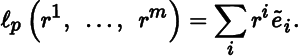
Let
be a semi‐Riemannian m‐manifold of index v, let p be a point in M, and let
be an orthonormal basis for Tp(M). Replacing ℝm with
in (18.10.1), we obtain the linear isomorphism
defined by
(19.7.2)
Using Theorem 14.1.6 and Theorem 14.2.5, let us now view
and
as semi‐Riemannian m‐manifolds of index v, and ℓp as a diffeomorphism.
Let
be a semi‐Riemannian manifold, and let p be a point in M. Let v and w be vectors in ℰp, and recall from (18.9.4) the differential map
The next result shows that dv(expp) can be viewed as a “linear isometry along radial geodesics”.
19.8 Riemann Curvature Tensor
Let
be a semi‐Riemannian manifold. In this setting, the curvature tensor (field) R, originally introduced in the context of smooth manifolds with a connection, is called the Riemann curvature tensor (field). We define a map
also called the Riemann curvature tensor (field) by
for all vector fields X, Y, Z, W in
.
Working through the details of Figure 19.5.1, Theorem 19.5.5(b), and Theorem 19.8.1, we find that ℛ can be identified with R. It is usual to think of ℛ as being obtained from R by “lowering an index”. This explains the practice of referring to both ℛ and R as the Riemann curvature tensor.
Let
be a semi‐Riemannian m‐manifold of index ν. We say that M is flat if for every point p in M, there is an isometry Fp :
, where V is a neighborhood of p in M, and U is an open set in
. According to Theorem 19.1.2, open sets in semi‐Riemannian manifolds are semi‐Riemannian manifolds in their own right, so this definition makes sense. The preceding conditions are not the same as requiring M to be locally isometric to
, because there is no guarantee that the Fp combine to give a smooth map from M to
.
The Riemann curvature tensor (in either of its manifestations) is a complicated mathematical object. The next result shows that in at least one instance, it has something explicitly geometric to say about “curvature”
19.9 Geodesics
In Section 18.8, a geodesic was defined to be a curve with zero acceleration. We now add to our knowledge of geodesics using the metric properties of semi‐Riemannian manifolds. In particular, we find a relationship between geodesics and length.
The next result demonstrates in a rigorous fashion the well‐known property of Euclidean space that the straight line segment joining any pair of distinct points is the shortest path between them.
Theorem 19.9.3 and the next result provide a dramatic illustration of how different the geometries of
and
are.
A generalization of Theorem 19.9.3 to arbitrary Riemannian manifolds is presented in Theorem 21.1.1. There is also a corresponding generalization of Theorem 19.9.5 to arbitrary Lorentz manifolds, but it is not included here.
19.10 Volume Forms
In Section 16.7, we discussed the integration of differential forms on smooth manifolds. The structure of semi‐Riemannian manifolds makes it possible to extend that theory to the integration of smooth functions.
Let
be an oriented semi‐Riemannian m‐manifold, let ΩM be its volume form, and let f be a function in C∞(M) that has compact support. Then fΩM is a form in Λm(M) that has compact support. The integral of f over M is defined by
The volume of M is obtained by taking f to be the function in C∞(M) with constant value 1:
19.11 orientation of Hypersurfaces
In this section, we summarize and extend some of the earlier results on the orientation of hypersurfaces.
Let
be an oriented semi‐Riemannian
‐manifold, where
, and let
be its volume form. Let
be a semi‐Riemannian hypersurface with boundary of
. We have from Theorem 17.1.5 that ∂M is a hypersurface of M. Suppose
is a semi‐Riemannian hypersurface of
. (We note that if
is Riemannian, then
and
are automatically Riemannian.) Our goal is to use the orientation of
to obtain an orientation of M, and in turn to use the orientation of M to find an orientation of ∂M.
We already have experience with this type of undertaking. To construct an orientation of M, suppose there is a nowhere‐tangent vector field V in
, and let
be the orientation of M induced by V. Then
is an oriented semi‐Riemannian hypersurface with boundary of
. Let ΩM be its volume form. It follows from Theorem 16.6.9 that: (i) for all points p in
is a basis for Tp(M) that is positively oriented with respect to
if and only if
is a basis for
that is positively oriented with respect to
, and (ii)
is an orientation form on M that induces
. According to Theorem 19.11.2(a),
.
By Theorem 17.2.5, there is an outward‐pointing vector field W in
. Let
be the (Stokes) orientation of ∂M induced by W. Then
is an oriented semi‐Riemannian hypersurface of
. Let Ω∂M be its volume form. It follows from Theorem 16.6.9 that: (iii) for all points q in
is a basis for Tq(∂M) that is positively oriented with respect to
if and only if
is a basis for Tq(M) that is positively oriented with respect to
, and (iv) iW(ΩM)|∂M is an orientation form on ∂M that induces
. Once again, according to Theorem 19.11.2(a), iW(ΩM)|∂M = Ω∂M. Combining (i) and (iii) gives (v): for all points q in
is a basis for Tq(∂M) that is positively oriented with respect to
if and only if
is a basis for
that is positively oriented with respect to
.
The key to the above construction is the existence of a nowhere‐tangent vector field in
. Unfortunately, there is no guarantee that such a vector field exists. This is evident from Example 12.7.9 when we view the Möbius band as a hypersurface of the Riemannian 3‐manifold
. The Möbius band has no shortage of nowhere‐tangent vector fields, but none of them is smooth.
Let us note that in the above discussion, we did not take advantage of the metric properties of
, or ∂M. This has special relevance to the existence of nowhere‐tangent vector fields: in the context of semi‐Riemannian manifolds, the premier nowhere‐tangent vector field is a unit normal vector field.
The next result is a generalization of Theorem 12.7.6.
We noted above that for smooth manifolds with boundary, Theorem 17.2.5 ensures the existence of an outward‐pointing smooth vector field along the boundary. In the more specialized setting of semi‐Riemannian manifolds, the outward‐pointing smooth vector field can be upgraded to a unit normal smooth vector field, as we now show.
We note that, taken together, parts (d) and (e) of the preceding theorem are consistent with Theorem 19.10.1. As an example of part (a), the outward‐pointing unit normal vector field for the unit sphere
is given by V(x, y, z) = (x, y, z), so
19.12 Induced Connections
In this section, we place the Euclidean derivative with respect to a vector field (Section 10.3) and the induced Euclidean derivative with respect to a vector field (Section 12.3) in the larger context of semi‐Riemannian manifolds.
Let
be a semi‐Riemannian
‐manifold, and let
be a semi‐Riemannian m‐submanifold, where
and ∇ are the Levi‐Civita connections. By definition,
and ∇ are maps
(19.12.1)
and
where
is the
‐module of smooth vector fields on
, and
is the C∞(M)‐module of smooth vector fields on M. Recall from Section 15.1 that
is the C∞(M)‐module of smooth vector fields along M, and that
is a C∞(M)‐submodule of
.
For each point p in M, we have by definition and (14.8.1) that
is nondegenerate on the subspace Tp(M) of
. By Theorem 4.1.3,
For brevity, let us denote the projection maps
and
by tanp and norp, respectively, so that
For each vector v in
, tanp(v) is a tangent vector at p, and norp(v) is a normal vector at p. We define the corresponding maps
by
for all points p in M and all vector fields V in
. Thus,
(19.12.2)
Let X and V be vector fields in
and
, respectively. As it stands,
is not meaningful because X and V are not in
. It can be shown that for each p in M, there is a chart
on
at p and vector fields
and
in
such that X and
agree on
, and likewise for V and
. Let us define
to be the restriction of
to
. In this way, we obtain a map
(9.12.3)
called the induced connection onM. Using the notation
in both (19.12.1) and (19.12.3) is intentional and meant to emphasize the relatedness of the two
maps. For a given vector field X in
, the induced covariant derivative with respect to X is the map
defined by
for all V in
. Corresponding to Theorem 12.3.1, we have the following result.
We have from (19.12.2) and the preceding two theorems that
which is the counterpart of (12.9.4).
For clarity in what follows, let us temporarily denote the above semi‐Riemannian connection
and induced semi‐Riemannian connection
by
and
, respectively. Let us similarly denote the Euclidean connection D and the induced Euclidean connection D by D1 and D2, respectively. The following table summarizes notation. In the above discussion of semi‐Riemannian connections, we began with
and ∇, and then constructed
. By contrast, in the case of the Euclidean connection, we began with D1 and D2, and then used Theorem 19.12.2 as a definition to construct ∇.