
Chapter 18
RISK AND RETURN
The spice of finance
Investors who buy financial securities face risks because they do not know with certainty the future selling price of their securities, nor the cash flows they will receive in the meantime. This chapter will try to explain and measure this risk, and also examine its repercussions.
Section 18.1 SOURCES OF RISK
There are various risks involved in financial securities, including:
- Industrial, commercial and labour risks, etc.
There are so many types of risk in this category that we cannot list them all here. They include lack of competitiveness, emergence of new competitors, technological breakthroughs, an inadequate sales network, strikes and so on. These risks tend to lower cash flow expectations and thus have an immediate impact on the value of the stock.
- Liquidity risk
This is the risk of not being able to sell an asset at its fair value as a result of either a liquidity discount or the complete absence of a market or buyers.
- Credit risk
This is the risk that a creditor will lose their entire investment if a debtor cannot repay them in full, even if the debtor's assets are liquidated. Traders call this counterparty risk.
- Foreign exchange (FX) risk
Fluctuations in exchange rates can lead to a loss of value of assets denominated in foreign currencies. Similarly, higher exchange rates can increase the value of debt denominated in foreign currencies when translated into the company's reporting currency base.
- Interest rate risk
The holder of financial securities is exposed to the risk of interest rate fluctuations. Even if the issuer fulfils their commitments entirely, there is still the risk of a capital loss or, at the very least, an opportunity loss.
- Systemic risk
This is the risk of collapse of the overall financial system through the bankruptcy chain and the domino effect linked to the interdependency of market players.
- Political risk
This includes risks created by a particular political situation or decisions by political authorities, such as nationalisation without sufficient compensation, revolution, exclusion from certain markets, discriminatory tax policies, inability to repatriate capital, etc.
- Regulatory risk
A change in the law or in regulations can directly affect the return expected in a particular sector. Pharmaceuticals, banks and insurance companies, among others, tend to be on the front lines here.
- Inflation risk
This is the risk that the investor will recover their investment with a depreciated currency, i.e. that they will receive a return below the inflation rate. A flagrant historical example is the hyperinflation in Germany in the 1920s.
- The risk of a fraud
This is the risk that some parties (internal or external) will lie or cheat. The most common examples are insider trading, CEO fraud or ransomware.
- Natural disaster risks
These include storms, earthquakes, volcanic eruptions, cyclones, tidal waves, etc., which destroy assets, or of a pandemic that stops the activity or restrains it a lot. The recent past has demonstrated that those risks cannot be neglected.
- Economic risk
This type of risk is characterised by bull or bear markets, anticipation of an acceleration or a slowdown in business activity or changes in labour productivity.
The list is nearly endless; however, at this point it is important to highlight two points:
- most financial analysis mentioned and developed in this book tends to generalise the concept of risk and highlight its impact on valuations, rather than analysing it in depth. So, given the extent to which markets are efficient and evaluate risk correctly, it is not necessary to redo what others have already done; and
- risk is always present. The so-called risk-free rate, to be discussed later, is simply a manner of speaking. Risk is always present, and to say that risk can be eliminated is either to be excessively confident or to be unable to think about the future – both very serious faults for an investor.
Obviously, any serious investment study should begin with a precise analysis of the risks involved.
The knowledge gleaned from analysts with extensive experience in the business, mixed with common sense, allows us to classify risks into two categories:
- economic risks (political, natural, inflation, fraud and other risks), which threaten cash flows from investments and which come from the “real economy”; and
- financial risks (liquidity, currency, interest rate and other risks), which do not directly affect cash flow, but nonetheless do come into the financial sphere. These risks are due to external financial events, and not to the nature of the issuer.
Section 18.2 RISK AND FLUCTUATION IN THE VALUE OF A SECURITY
All of the aforementioned risks can penalise the financial performance of companies and their future cash flows. Obviously, if a risk materialises that seriously hurts company cash flows, then investors will seek to sell their securities. Consequently, the value of the security falls.
Moreover, if a company is exposed to significant risk, then some investors will be reluctant to buy its securities. Even before risk materialises, investors' perceptions that a company's future cash flows are uncertain or volatile will serve to reduce the value of its securities.
Most modern finance is based on the premise that investors seek to reduce the uncertainty of their future cash flows. By its very nature, risk increases the uncertainty of an asset's future cash flow, and it therefore follows that such uncertainty will be priced into the market value of a security.
Investors consider risk only to the extent that it affects the value of the security. Risks can affect value by changing anticipations of cash flows or the rate at which these cash flows are discounted.
To begin with, it is important to realise that in corporate finance no fundamental distinction is made between the risk of asset revaluation and the risk of asset devaluation.
That is to say, whether investors expect the value of an asset to rise (upside) or decrease (downside) is immaterial.1 It is the fact that risk exists in the first place that is of significance and affects how investors behave.
Consider, for example, a security with the following cash flows expected for years 1 to 4:
| Year | 1 | 2 | 3 | 4 |
|---|---|---|---|---|
| Cash flow (in €) | 100 | 120 | 150 | 190 |
Imagine the value of this security is estimated to be €2,000 in five years. Assuming a 9% discounting rate, its value today would be:
If a sudden sharp rise in interest rates raises the discounting rate to 13%, the value of the security becomes:
The security's value has fallen by 15% whereas cash flows have not changed.
However, if the company comes out with a new product that raises projected cash flow by 20%, with no further change in the discounting rate, the security's value then becomes:
The security's value increases for reasons specific to the company, not because of a fall of interest rates in the market.
Now, suppose that there is an improvement in the overall economic outlook that lowers the discounting rate to 10%. If there is no change in expected cash flows, the stock's value would be:
Again, there has been no change in the stock's intrinsic characteristics and yet its value has risen by 12%.
If there is stiff price competition, then previous cash flow projections will have to be adjusted downward by 10%. If all cash flows fall by the same percentage and the discounting rate remains constant, the value of the company becomes:
Once again, the security's value decreases for reasons specific to the company, not because of a fall in the market.
In the previous example, a European investor would have lost 10% of their investment (from €2,009 to €1,808). If, in the interim, the euro had risen from $1.10 to $1.31, a US investor would have gained 7% (from $2,210 to $2,365).
A closer analysis shows that some securities are more volatile than others, i.e. their price fluctuates more widely. We say that these stocks are “riskier”. The riskier a stock is, the more volatile its price, and vice versa. Conversely, the less risky a security is, the less volatile its price, and vice versa.
Volatility can be measured mathematically by variance and standard deviation.
Typically, it is safe to assume that risk dissipates over the long term. The erratic fluctuations in the short term give way to the clear outperformance of equities over bonds, and bonds over money-market investments. The chart below tends to back up this point of view. It presents data on the path of wealth (POW) for the three asset classes. The POW measures the growth of €1 invested in any given asset, assuming that all proceeds are reinvested in the same asset.
As is easily seen from the chart, risk does dissipate, but only over the long term. In other words, an investor must be able to invest their funds and then do without them during this long-term timeframe. It sometimes requires strong nerves not to give in to the temptation to sell when prices collapse, as happened with stock markets in 1929, 1974, 2001, 2008, or 2011.
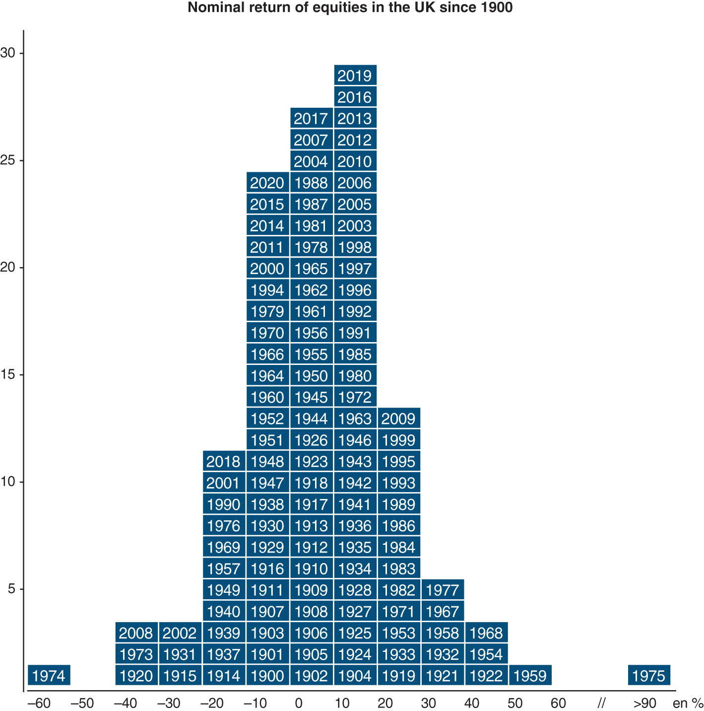
Since 1900, UK stocks have delivered an average annual return after inflation of 5.4%. Yet, during 39 of those years the returns were negative, in particular in 1974, when investors lost 57% on a representative portfolio of UK stocks.
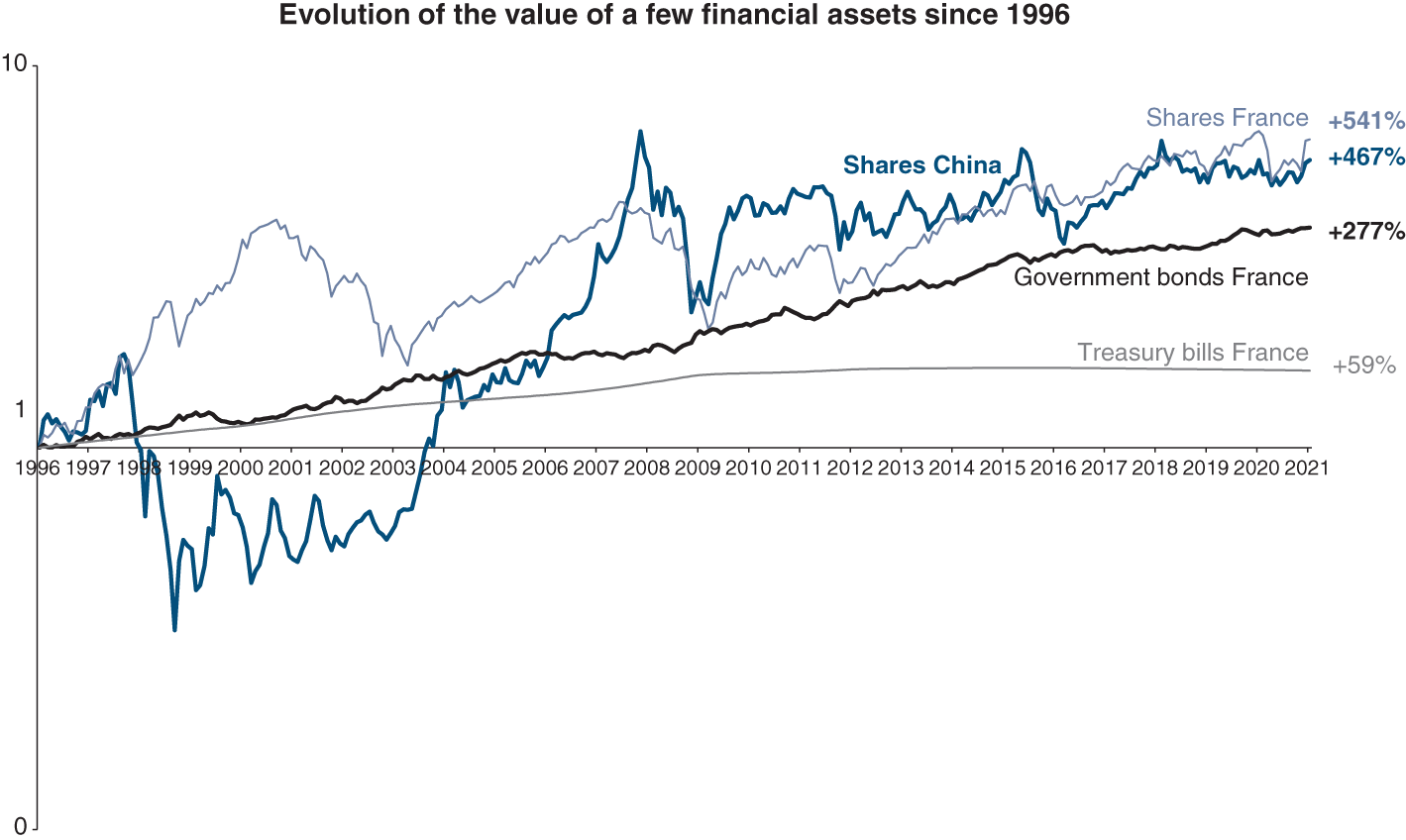
Source: Data from Factset
Source: Based on Dimson, Marsh and Staunton (2020)
And in worst-case scenarios, it must not be overlooked that some financial markets vanished entirely, including the Russian equity market after the 1917 revolution, the German bond market with the hyperinflation of 1921–1923, the Japanese and German equity markets in 1945, and the Chinese equity market in 1949. Over the stretch of one century, these may be exceptional events, but they have enormous repercussions when they do occur.
Section 18.3 TOOLS FOR MEASURING RETURN AND RISK
1/ EXPECTED RETURN
To begin, it must be realised that a security's rate of return and the value of a financial security are actually two sides of the same coin. The rate of return will be considered first.
The holding-period return is calculated from the sum total of cash flows for a given investment, i.e. income, in the form of interest or dividends earned on the funds invested and the resulting capital gain or loss when the security is sold.
If just one period is examined, then the return on a financial security can be expressed as follows:
Here, F1 is the income received by the investor during the period, V0 is the value of the security at the beginning of the period and V1 is the value of the security at the end of the period.
In an uncertain world, investors cannot calculate their returns in advance, as the value of the security is unknown at the end of the period. In some cases, the same is true for the income to be received during the period.
Therefore, investors use the concept of expected return, which is the average of possible returns weighted by their likelihood of occurring. Familiarity with the science of statistics should aid in understanding the notion of expected outcome.
Given security A with 12 chances out of 100 of showing a return of −22%, 74 chances out of 100 of showing a return of 6% and 14 chances out of 100 of showing a return of 16%, its expected return would then be:
More generally, expected return or expected outcome is equal to:
where rt is a possible return and pt the probability of it occurring.
2/ STANDARD DEVIATION, A RISK-ANALYSIS TOOL
Intuitively, the greater the risk on an investment, the wider the variations in its return, and the more uncertain that return is. While the holder of a government bond is sure to receive their coupons (unless the government goes bankrupt!), this is far from true for the shareholder of a biotech company. They could lose everything, show a decent return or hit the jackpot.
Therefore, the risk carried by a security can be looked at in terms of the dispersion of its possible returns around an average return. Consequently, risk can be measured mathematically by the variance of its return, i.e. by the sum of the squares of the deviation of each return from expected outcome, weighted by the likelihood of each of the possible returns occurring, or:
Standard deviation in returns is the most often used measure to evaluate the risk of an investment. Standard deviation is expressed as the square root of the variance:
The variance of investment A above is therefore:
where V(r) = 1%, which corresponds to a standard deviation of 10%.
Section 18.4 MARKET AND SPECIFIC RISK
Risk in finance is materialised by fluctuation of value, which is equivalent to fluctuation of returns. Hence, one figure summarises all of the different risks, the knowledge of which does not really matter. Only the impact on value is important.
Fluctuations in the value of a security can be due to:
- fluctuations in the entire market. The market could rise as a whole after an unexpected cut in interest rates, stronger-than-expected economic growth figures, etc. All stocks will then rise, although some will move more than others. The same thing can occur when the entire market moves downward; or
- factors specific to the company that do not affect the market as a whole, such as a major order, the bankruptcy of a competitor, a new regulation affecting the company's products, a scandal over fraud on product tests, discovering contaminated products, etc.
These two sources of fluctuation produce two types of risk: market risk and specific risk.
- Market, systematic or undiversifiable risk is due to trends in the entire economy, tax policy, interest rates, inflation, etc. Remember, this is the risk of the security correlated to market risk. To varying degrees, market risk affects all securities. For example, if a nation switches to a 35-hour working week with no adjustment in wages, all companies will be affected. However, in such a case, it stands to reason that textile makers will be affected more than cement companies.
- Specific, intrinsic or idiosyncratic risk is independent of market-wide phenomena and is due to factors affecting just the one company, such as mismanagement, a factory fire, an invention that renders a company's main product line obsolete, etc. (In the next chapter, it will be shown how this risk can be eliminated by diversification, a reason why this risk is also sometimes call diversifiable risk.)
Market volatility can be economic or financial in origin, but it can also result from anticipation of flows (dividends, capital gains, etc.) or a variation in the cost of equity. For example, an overheating of the economy could raise the cost of equity (i.e. after an increase in the central bank rate) and reduce anticipated cash flows due to weaker demand. Together, these two factors could exert a double downward pressure on financial securities.
Since market risk and specific risk are independent, they can be measured independently and we can apply Pythagoras's theorem (in more mathematical terms, the two risk vectors are orthogonal) to the overall risk of a single security:
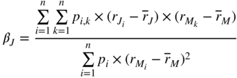
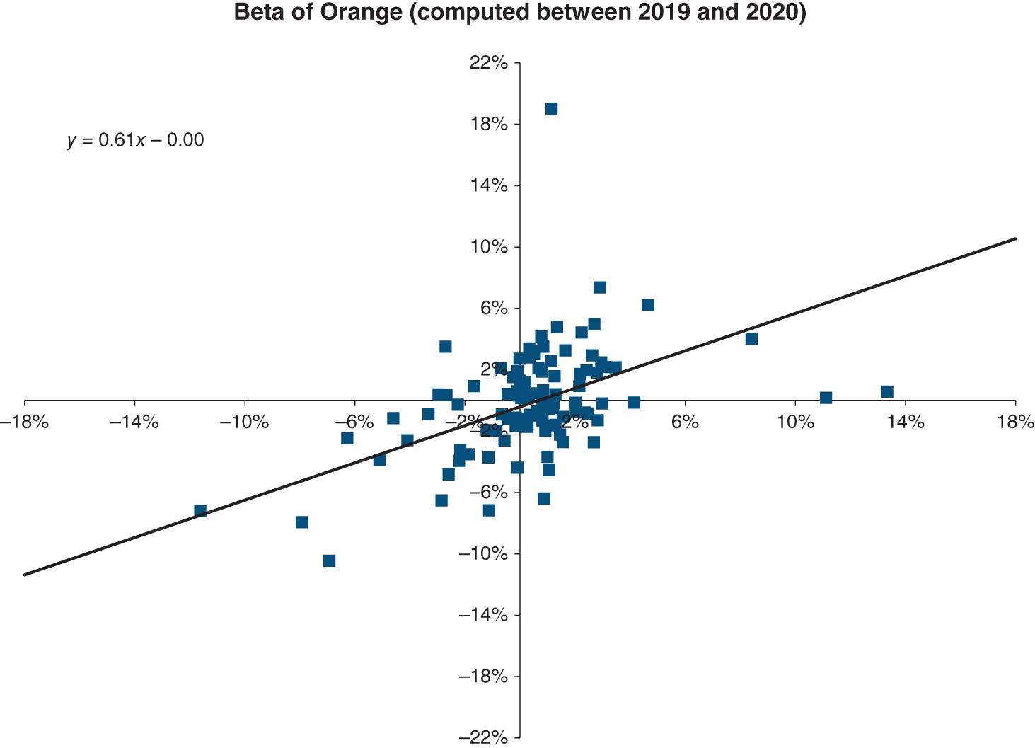
The systematic risk presented by a financial security is frequently expressed in terms of its sensitivity to market fluctuations. This is done via a linear regression between periodic market returns (rMt) and the periodic returns of each security J: rJt. This yields the regression line expressed in the following equation:
βJ is a parameter specific to each investment J and it expresses the relationship between fluctuations in the value of J and the market. It is thus a coefficient of volatility or of sensitivity. We call it the beta or the beta coefficient.
A security's total risk is reflected in the standard deviation of its return, s(rJ).
A security's market risk is therefore equal to βJ × σ(rM), where σ(rM) is the standard deviation of the market return. Therefore it is also proportional to the beta, i.e. the security's market-linked volatility. The higher the beta, the greater the market risk borne by the security. If β >1, then the security's returns move at a ratio of greater than 1:1 with respect to the market. Conversely, securities whose beta is below 1 are less affected by market fluctuations.
The specific risk of security J is equal to the standard deviation of the different residuals εJ of the regression line, expressed as σ(εJ), i.e. the variations in the stock that are not tied to market variations.
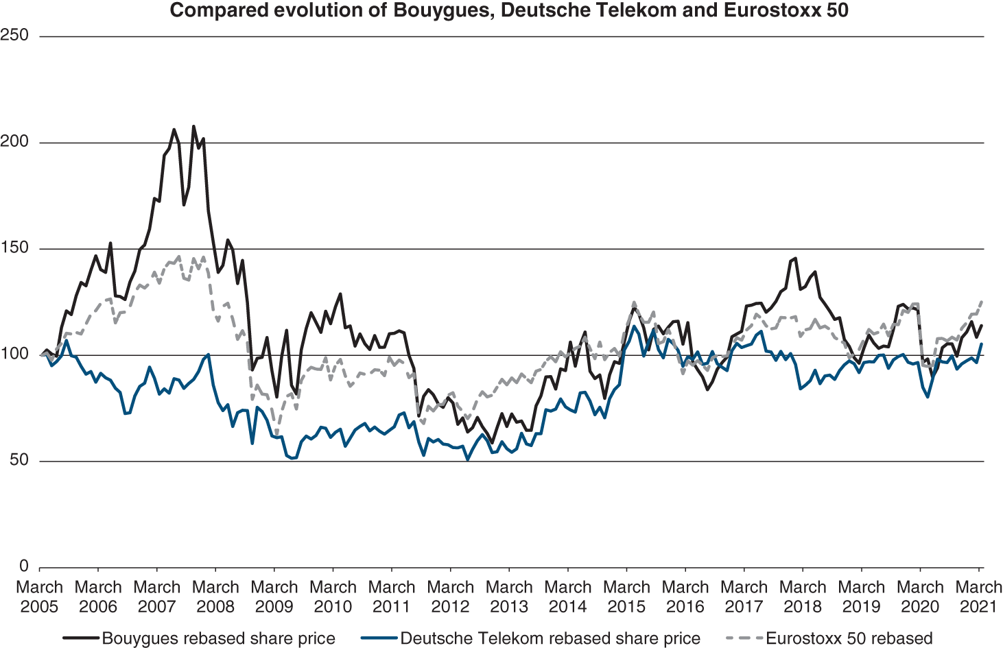
This chart shows that the β of Bouygues is higher than that of Deutsche Telekom.
Source: Data from Factset
This can be expressed mathematically as follows:
Section 18.5 THE BETA COEFFICIENT
1/ CALCULATING BETA
β measures a security's sensitivity to market risk. For security J, it is mathematically obtained by performing a regression analysis of security returns versus market returns.
Hence:

Here, Cov(rJ, rM) is the covariance of the return of security J with that of the market, and V(rM) is the variance of the market return. This can be represented as:
More intuitively, β corresponds to the slope of the regression of the security's return versus that of the market. The line we obtain is defined as the characteristic line of a security.
As an example, we have calculated the β for Orange and it stands at 0.61.
The β of Orange used to be higher in the late 1990s (1.83). The stock was more volatile than the market, its market risk was high. With the mobile telecom and Internet market maturing, the industry became less risky and the β of Orange is now 1, as shown in the following graph:
Source: Data from Factset
2/ PARAMETERS BEHIND BETA
By definition, the market β is equal to 1. β of fixed-income securities ranges from about 0 to 0.5. The β of equities is usually higher than 0.5, and normally between 0.5 and 1.5. We are not aware of any simple investment products with a negative β, and shares with a β greater than 2 are quite exceptional.
To illustrate, the table below presents betas, as of 2019, of the members of the Euro Stoxx 50 index:
| Beta of the Eurostoxx 50 | |||||||||
|---|---|---|---|---|---|---|---|---|---|
| Linde | 0.47 | L'Oréal | 0.76 | SAP | 0.92 | Siemens | 1.07 | AXA | 1.21 |
| Royal Ahold Delhaize | 0.59 | Inditex | 0.76 | AB InBev | 0.92 | Bayer | 1.10 | ASML | 1.27 |
| Amadeus | 0.61 | Unilever | 0.77 | Vivendi | 0.92 | Telefonica | 1.12 | Volkswagen | 1.35 |
| Danone | 0.68 | Eni | 0.79 | Deutsche Post | 0.97 | Philips | 1.12 | ING | 1.38 |
| Deutsche Telekom | 0.68 | Adidas | 0.81 | Total | 0.97 | Daimler | 1.15 | BNP Paribas | 1.39 |
| EssilorLuxottica | 0.69 | Unibail-Rodamco-Westfield | 0.82 | Fresenius | 1.01 | Airbus | 1.16 | Nokia | 1.40 |
| Orange | 0.72 | Munich Re | 0.82 | Safran | 1.03 | LVMH | 1.17 | BBVA | 1.42 |
| Sanofi | 0.72 | Vinci | 0.87 | Allianz | 1.03 | Kering | 1.18 | Société Générale | 1.46 |
| Iberdrola | 0.75 | Engie | 0.88 | BMW | 1.06 | Schneider | 1.21 | Intesa Sanpaolo | 1.46 |
| Enel | 0.75 | Air Liquide | 0.91 | BASF | 1.07 | CRH | 1.21 | Santander | 1.56 |
Source: Factset, 2019
For a given security, the following parameters explain the value of beta:
(a) Sensitivity of the stock's sector to the state of the economy
The greater the effect of the state of the economy on a business sector, the higher its β is – temporary work is one such highly exposed sector. Another example is automakers, which tend to have a β close to 1. There is an old saying in North America, “As General Motors goes, so goes the economy”. This serves to highlight how GM's financial health is to some extent a reflection of the health of the entire economy. Thus, beta analysis can show how GM will be directly affected by macroeconomic shifts.
(b) Cost structure
The greater the proportion of fixed costs to total costs, the higher the breakeven point, and the more volatile the cash flows. Companies that have a high ratio of fixed costs (such as cement makers) have a high β, while those with a low ratio of fixed costs (such as mass-market service retailers) have a low β.
(c) Financial structure
The greater a company's debt, the greater its financing costs. Financing costs are fixed costs which increase a company's breakeven point and, hence, its earnings volatility. The heavier a company's debt or the more heavily leveraged the company is, the higher the β of its shares is.
(d) Visibility on company performance
The quality of management and the clarity and quantity of information the market has about a company will all have a direct influence on its beta. All other factors being equal, if a company gives out little or low-quality information, the β of its stock will be higher as the market will factor the lack of visibility into the share price.
(e) Earnings growth
The higher the forecast rate of earnings growth, the higher the β. Most of a company's value in cash flows is far down the road and thus highly sensitive to any change in assumptions.
Section 18.6 PORTFOLIO RISK
1/ THE FORMULA APPROACH
Consider the following two stocks, Heineken and Criteo, which have the following characteristics:
| Heineken % | Criteo % | |
|---|---|---|
| Expected return: E(r) | 6 | 13 |
| Risk: σ(r) | 10 | 17 |
As is clear from this table, Criteo offers a higher expected return while presenting a greater risk than Heineken. Inversely, Heineken offers a lower expected return but also presents less risk.
These two investments are not directly comparable. Investing in Criteo means accepting more risk in exchange for a higher return, whereas investing in Heineken means playing it relatively safe.
Therefore, there is no clear-cut basis by which to choose between Criteo and Heineken. However, the problem can be looked at in another way: would buying a combination of Criteo and Heineken shares be preferable to buying just one or the other?
It is likely that the investor will seek to diversify and create a portfolio made up of Criteo shares (in a proportion of XC) and Heineken shares (in a proportion of XH). This way, they will expect a return equal to the weighted average return of each of these two stocks, or:
where XC + XH = 1.
Depending on the proportion of Criteo shares in the portfolio (XC), the portfolio would look like this:
| XC (%) | 0 | 25 | 33.3 | 50 | 66.7 | 75 | 100 |
| E(rH,C) (%) | 6 | 7.8 | 8.3 | 9.5 | 10.7 | 11.3 | 13 |
The portfolio's variance is determined as follows:
where Cov(rH, rC) is the covariance. It measures the degree to which Heineken and Criteo fluctuate together. It is equal to:
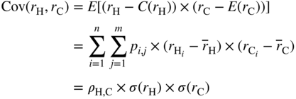
Here, pi,j is the probability of joint occurrence and ρH,C is the correlation coefficient of returns offered by Heineken and Criteo. The correlation coefficient is a number between −1 (where the correlation between returns on the two stocks will be perfectly negative) and 1 (where the correlation between returns on the two stocks will be perfectly positive). Correlation coefficients are usually positive, as most stocks rise together in a bullish market and fall together in a bearish market.
By plugging the variables back into our variance equation above, we obtain:
Given that:
it is therefore possible to say:
or:
Therefore, the overall risk of a portfolio consisting of Criteo and Heineken shares is less than the weighted average of the risks of the two stocks.
Assuming that ρH,C is equal to 0.5 (from the figures in the above example), we obtain the following:
| X (%) | 0 | 25 | 33.3 | 50 | 66.7 | 75 | 100 |
| σ(rH,C) (%) | 10.0 | 10.3 | 10.7 | 11.8 | 13.3 | 14.2 | 17.0 |
Hence, a portfolio consisting of 50% Criteo and 50% Heineken has a standard deviation of 11.8% or less than the average of Criteo and Heineken, which is (50% × 17%) + (50% × 10%) = 13.5%.
On a chart, it looks like this:
Only a correlation coefficient of 1 creates a portfolio risk that is equal to the average of its component risks.
CORRELATION BETWEEN DIFFERENT STOCK MARKETS (2014–2019)
| Brazil | China | France | Germany | Morocco | Switzerland | UK | United States | |
|---|---|---|---|---|---|---|---|---|
| Brazil | 1.00 | 0.30 | 0.68 | 0.67 | 0.82 | 0.38 | 0.72 | 0.90 |
| China | 0.30 | 1.00 | 0.66 | 0.70 | 0.44 | 0.52 | 0.36 | 0.47 |
| France | 0.68 | 0.66 | 1.00 | 0.97 | 0.78 | 0.69 | 0.82 | 0.84 |
| Germany | 0.67 | 0.70 | 0.97 | 1.00 | 0.84 | 0.63 | 0.84 | 0.83 |
| Morocco | 0.82 | 0.44 | 0.78 | 0.84 | 1.00 | 0.40 | 0.83 | 0.85 |
| Switzerland | 0.38 | 0.52 | 0.69 | 0.63 | 0.40 | 1.00 | 0.54 | 0.46 |
| UK | 0.72 | 0.36 | 0.82 | 0.84 | 0.83 | 0.54 | 1.00 | 0.77 |
| United States | 0.90 | 0.47 | 0.84 | 0.83 | 0.85 | 0.46 | 0.77 | 1.00 |
Source: Data from Factset
Emerging markets still bring diversification and are more correlated among themselves than with developed countries.
However, sector diversification is still highly efficient thanks to the low correlation coefficients among different industries:
CORRELATION BETWEEN ECONOMIC SECTORS WORLDWIDE (2014–2019)
| Sector | Banks | Automotive | Pharmaceuticals & Biotech | Oil & Gas | Construction | Softwares | Energy | Agriculture & Food chain | Retailing | Metals & Mining | Aerospace & Defence |
|---|---|---|---|---|---|---|---|---|---|---|---|
| Banks | 1.00 | 0.75 | 0.52 | 0.35 | 0.66 | 0.74 | 0.26 | 0.56 | 0.66 | 0.71 | 0.79 |
| Automotive | 0.75 | 1.00 | 0.49 | 0.24 | 0.43 | 0.28 | 0.21 | 0.31 | 0.24 | 0.38 | 0.35 |
| Pharmaceuticals & Biotech | 0.52 | 0.49 | 1.00 | −0.20 | 0.54 | 0.57 | −0.30 | 0.73 | 0.64 | 0.00 | 0.56 |
| Oil & Gas | 0.35 | 0.24 | −0.20 | 1.00 | −0.25 | 0.04 | 0.99 | −0.25 | −0.03 | 0.79 | 0.11 |
| Construction | 0.66 | 0.43 | 0.54 | −0.25 | 1.00 | 0.77 | −0.34 | 0,89 | 0,74 | 0,24 | 0.76 |
| Softwares | 0.74 | 0.28 | 0.57 | 0.04 | 0.77 | 1.00 | −0.10 | 0.78 | 0.97 | 0.48 | 0.99 |
| Energy | 0.26 | 0.21 | −0.30 | 0.99 | −0.34 | −0.10 | 1.00 | −0.36 | −0.16 | 0.72 | −0.02 |
| Agriculture & Food chain | 0.56 | 0.31 | 0.73 | −0.25 | 0.89 | 0.78 | −0.36 | 1.00 | 0.78 | 0.15 | 0.76 |
| Retailing | 0.66 | 0.24 | 0.64 | −0.03 | 0.74 | 0.97 | −0.16 | 0.78 | 1.00 | 0.36 | 0.95 |
| Metals & Mining | 0.71 | 0.38 | 0.00 | 0.79 | 0.24 | 0.48 | 0.72 | 0.15 | 0.36 | 1.00 | 0.55 |
| Aerospace & Defence | 0.79 | 0.35 | 0.56 | 0.11 | 0.76 | 0.99 | −0.02 | 0.76 | 0.95 | 0.55 | 1.00 |
Source: Data from Factset
Section 18.7 CHOOSING AMONG SEVERAL RISKY ASSETS AND THE EFFICIENT FRONTIER
This section will address the following questions: why is it correct to say that the beta of an asset should be measured in relation to the market portfolio? Above all, what is the market portfolio?
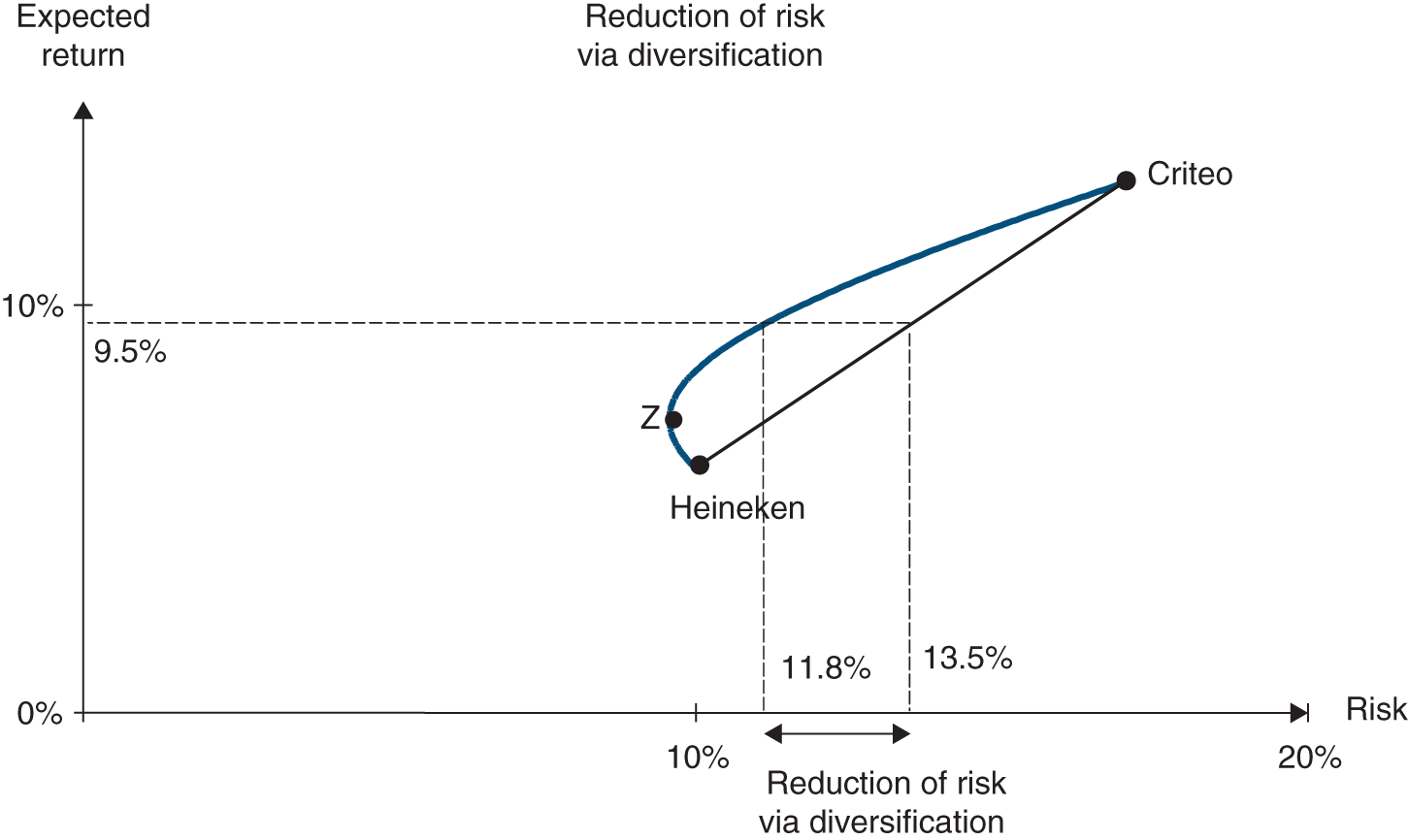
To begin, it is useful to study the impact of the correlation coefficient on diversification. Again, the same two securities will be analysed: Criteo (C) and Heineken (H). By varying ρH,C between −1 and +1, we obtain:
| Proportion of C shares in portfolio (XC) (%) | 0 | 25 | 33.3 | 50 | 66.7 | 75 | 100 | |
|---|---|---|---|---|---|---|---|---|
| Return on the portfolio: E(rH,C) (%) | 6.0 | 7.8 | 8.3 | 9.5 | 10.7 | 11.3 | 13.0 | |
| Portfolio risk σ(rH,C) (%) | ρH,C = −1 | 10.0 | 3.3 | 1.0 | 3.5 | 8.0 | 10.3 | 17.0 |
| ρH,C = −0.5 | 10.0 | 6.5 | 6.2 | 7.4 | 10.1 | 11.7 | 17.0 | |
| ρH,C = 0 | 10.0 | 8.6 | 8.7 | 9.9 | 11.8 | 13.0 | 17.0 | |
| ρH,C = 0.3 | 10.0 | 9.7 | 10.0 | 11.1 | 12.7 | 13.7 | 17.0 | |
| ρH,C = 0.5 | 10.0 | 10.3 | 10.7 | 11.8 | 13.3 | 14.2 | 17.0 | |
| ρH,C = 1 | 10.0 | 11.8 | 12.3 | 13.5 | 14.7 | 15.3 | 17.0 |
Note the following caveats:
- If Criteo and Heineken were perfectly correlated (i.e. the correlation coefficient was 1), then diversification would have no effect. All possible portfolios would lie on a line linking the risk/return point of Criteo with that of Heineken. Risk would increase in direct proportion to Criteo's stock added.
- If the two stocks were perfectly inversely correlated (correlation coefficient −1), then diversification would be total. However, there is little chance of this occurring, as both companies are exposed to the same economic conditions.
- Generally speaking, Criteo and Heineken are positively, but imperfectly, correlated and diversification is based on the desired amount of risk.
With a fixed correlation coefficient of 0.3, there are portfolios that offer different returns at the same level of risk. Thus, a portfolio consisting of two-thirds Heineken and one-third Criteo shows the same risk (10%) as a portfolio consisting of just Heineken, but returns 8.3% versus only 6% for Heineken.
There is no reason for an investor to choose a given combination if another offers a better (efficient) return at the same level of risk.
Efficient portfolios (such as a combination of Criteo and Heineken shares) offer investors the best risk–return ratio (i.e. minimum risk for a given return).
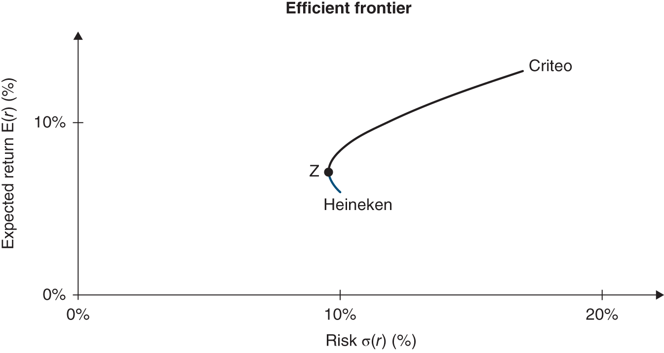
For any portfolio that does not lie on the efficient frontier, another can be found that, given the level of risk, offers a greater return or that, at the same return, entails less risk.
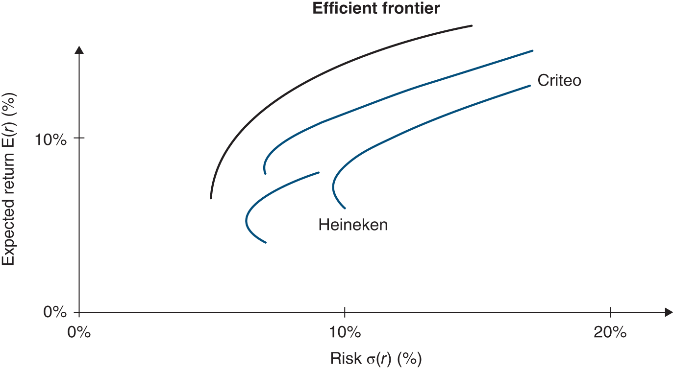
With a larger number of stocks, i.e. more than just two, the investor can improve their efficient frontier, as shown in the following chart.
Section 18.8 CHOOSING BETWEEN SEVERAL RISKY ASSETS AND A RISK-FREE ASSET: THE CAPITAL MARKET LINE
1/ RISK-FREE ASSETS
By definition, risk-free assets are those whose returns, the risk-free rate (rF), are certain. The standard deviation of their return is thus zero. Traditionally, this is illustrated with government bonds, although we can no longer assume that the government cannot go bankrupt, given the high levels of debt in many countries. This has now led us to view the 1-month Treasury bill as risk-free (e.g. the German bill for the Eurozone, the US Treasury bill for the US).
If a portfolio has a risk-free asset F in proportion (1 − XH) and the portfolio consists exclusively of Heineken shares, then the portfolio's expected return E(rH,F) will be equal to:
The portfolio's expected return is equal to the return of the risk-free asset, plus a risk premium, multiplied by the proportion of Heineken shares in the portfolio. The risk premium is the difference between the expected return on Heineken and the return on the risk-free asset.
How much risk does the portfolio carry? Its risk will simply be the risk of the Heineken stock, commensurate with its proportion in the portfolio, expressed as follows:
If investors want to increase their expected return, they will increase XH. They could even borrow money at the risk-free rate and use the funds to buy Heineken stock, but the risk carried by their portfolio would rise commensurately.
By combining the previous two equations, we can eliminate XH, thus deriving the following equation:

Continuing with the Heineken example, and assuming that rF is 3%, with 50% of the portfolio consisting of a risk-free asset, the following is obtained:

Hence:
For a portfolio that includes a risk-free asset, there is a linear relationship between expected return and risk. To lower a portfolio's risk, simply liquidate some of the portfolio's stock and put the proceeds into a risk-free asset. To increase risk, it is only necessary to borrow at the risk-free rate and invest in a stock with risk.
2/ RISK-FREE ASSETS AND THE EFFICIENT FRONTIER
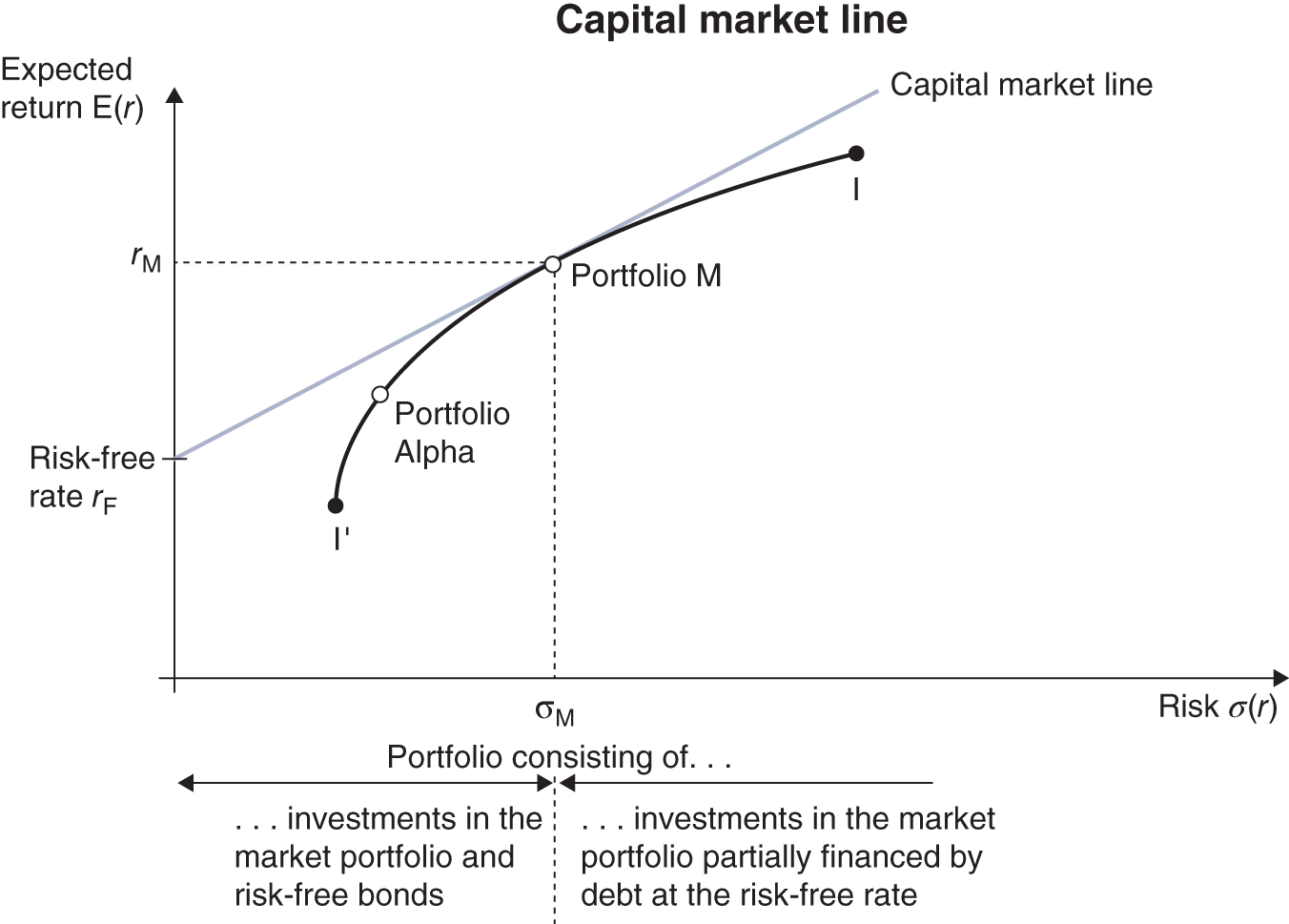
The risk–return profile can be chosen by combining risk-free assets and a stock portfolio (the alpha portfolio on the chart below). This new portfolio will be on a line that connects the risk-free rate to the portfolio alpha that has been chosen. But as we can observe on the chart, this portfolio is not the best portfolio. Portfolio P provides a better return for the same risk. Portfolio P is situated on the line tangential to the efficient frontier. There is no other portfolio than P that offers a better return for the same amount of risk-taking. What is portfolio P made up of? It's made up of a combination of the portfolio of risky assets M (located on the efficient frontier at the tangential point with the line originating from the risk-free rate) and the risk-free asset.
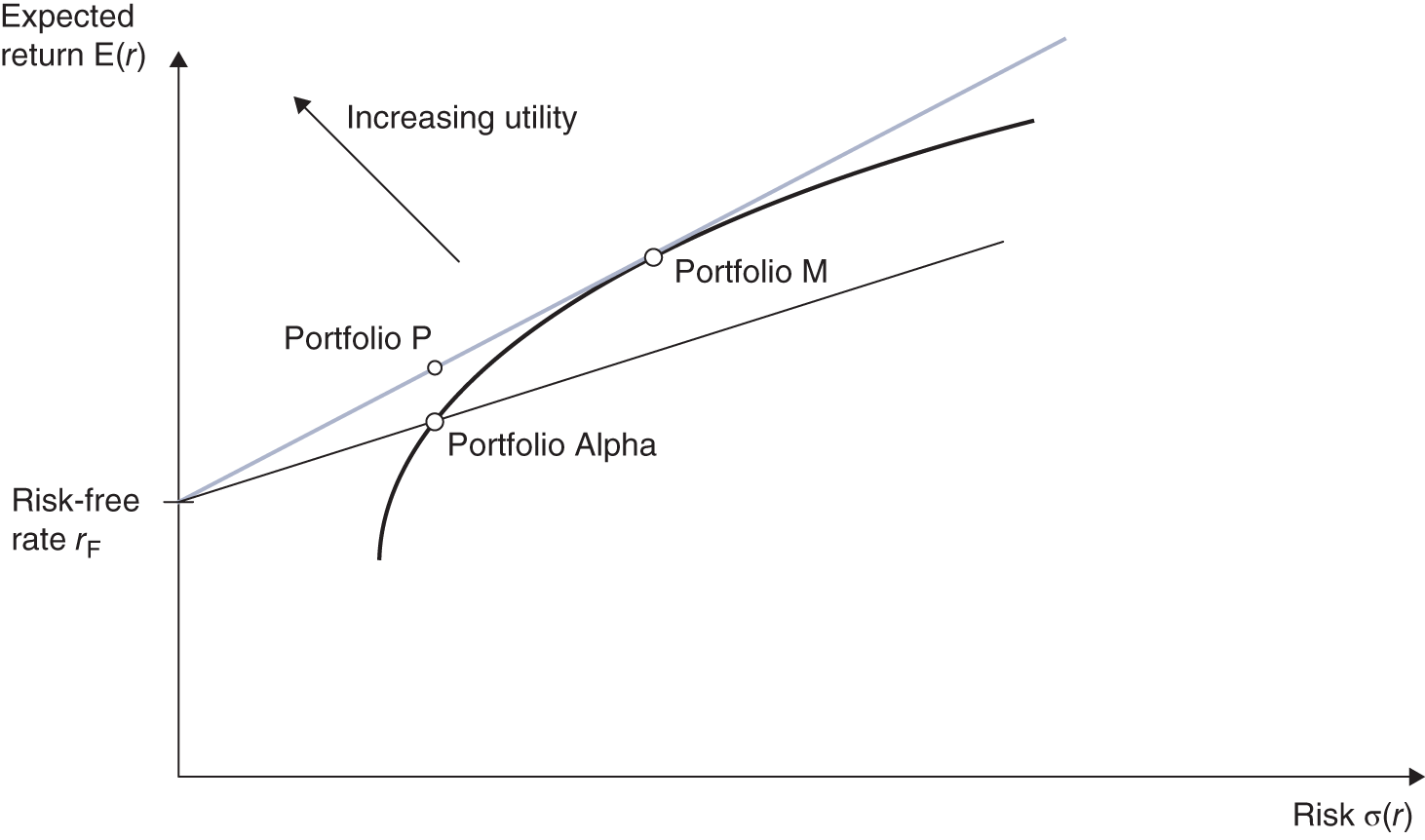
Investors' taste for risk can vary, yet the above graph demonstrates that the shrewd investor should be investing in portfolio M. It is then a matter of adjusting the risk exposure by adding or subtracting risk-free assets.
If all investors acquire the same portfolio, then this portfolio must contain all existing shares. To understand why, suppose that stock i was not in portfolio M. In that case, nobody would want to buy it, since all investors hold portfolio M. Consequently, there would be no market for it and it would cease to exist.
The weighting of stock i in a market portfolio will necessarily be the value of the single security divided by the sum of all the assets. As we are assuming fair value, this will be the fair value of i.
3/ CAPITAL MARKET LINE
The expected return of a portfolio consisting of the market portfolio and the risk-free asset can be expressed by the following equation:
where E(rP) is the portfolio's expected return, rF the risk-free rate, E(rM) the return on the market portfolio, σP the portfolio's risk and σM the risk of the market portfolio.
This is the equation of the capital market line.
The most efficient portfolios in terms of return and risk will always be on the capital market line. The tangent point at M constitutes the optimal combination for all investors. If we introduce the assumption that all investors have homogeneous expectations, i.e. that they have the same opinions on expected returns and risk of financial assets, then the efficient frontier of risky assets will be the same for all of them. The capital market line is the same for all investors and thus each of them would hold a combination of the portfolio M and the risk-free asset.
It is reasonable to say that the portfolio M includes all the assets weighted for their market capitalisation. This is defined as the market portfolio. The market portfolio is the portfolio that all investors hold a fraction of, proportional to the market's capitalisation.
Section 18.9 HOW PORTFOLIO MANAGEMENT WORKS
The financial theory described so far seems to give a clear suggestion: in efficient markets, invest only in highly diversified mutual funds and in government bonds.
The asset management industry is one of the most important industries in the modern economy, managing €55,000bn worldwide (40% of this amount being invested in shares and 22% in bonds, the rest in short-term debts and multi-assets). Managers are employees of banks, insurance companies or independent.
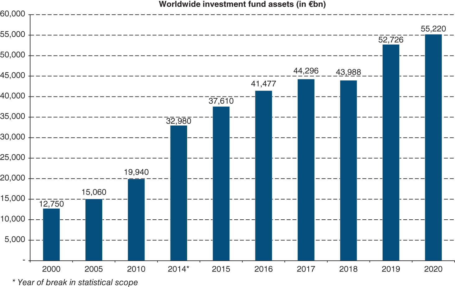
Source: Data from Efama
However, as our readers know, not all investors subscribe to this theory. Some take other approaches, described below. Sometimes investors combine different approaches.
The strategy that is closest to financial theory is index tracking, also known as passive management. It consists of trying to follow the performance of a market index. Index trackers are ideal tools for the investor who believes strongly in market efficiency. They also benefit from scale effect and therefore have reduced operating costs. Index trackers can be listed on a market and are then called exchange-traded funds (ETFs). Most stock markets now have a specific market segment for the listing of trackers. Across global markets, over 7,845 trackers are listed for a total amount of over $8,331bn.
In terms of portfolio management, we shall consider the difference between a top-down and a bottom-up approach. In a top-down approach, investors focus on the asset class (shares, bonds, money-market funds) and the international markets in which they wish to invest (i.e. the individual securities chosen are of little importance). In a bottom-up approach (commonly known as stock-picking), investors choose stocks on the basis of their specific characteristics, not the sector in which they belong. The goal of the bottom-up approach is to find that rare pearl, i.e. the stock that is undervalued by the market, which is identified through fundamental analysis, a method of seeking the intrinsic value of a stock. Investors following this approach believe that sooner or later, market value will approach intrinsic value.
These stocks can be growth stocks, i.e. companies who are operating in a fast-growing industry; or value stocks, i.e. firms operating in more mature sectors but which offer long-term performance. At the opposite end you will find yield stocks whose return comes almost exclusively from the dividend paid, and their market price is then pretty stable.
Investors who focus on technical analysis, the so-called chartists, do not seek to determine the value of a stock. Instead, these investors conduct detailed studies of trends in a stock's market value and transaction volumes in the hope of spotting short-term trends.
Another type of fund management has arisen since the mid-1990s, so-called alternative management, which gives itself total freedom of investment tools, whether listed or not: equities, bonds, currencies, commodities, etc., and of investment styles: buying, short selling, derivatives (see Chapter 23), heavy reliance on debt, and shareholder activism. Its objective is not to duplicate the performance of any index, but to obtain positive returns regardless of the state of the market and thus to offer additional diversification. An example of alternative management is the hedge fund, which is a speculative fund seeking high returns and relying heavily on derivatives, and options in particular. Hedge funds use leverage and commit capital in excess of their equity.
At the beginning of 2021, over 7,000 hedge funds were active in the world and had about $3,800bn under management.
In recent years, hedge funds' risk-adjusted performance has been above that of traditional management, this even in bearish markets, with a relatively low correlation with other investment opportunities.
Hedge funds may present some restrictions on investing (minimum size). Funds of funds allow a larger number of investors to invest in hedge funds. The funds of funds pick up the best hedge fund managers and package their products to be offered to a wide number of investors.
Last but not least are private equity funds, which invest mainly in non-listed firms at different stages of maturity, via LBOs or otherwise (see Chapter 47). Their growing scope of investments is slowly turning them into an alternative to stock markets.
Regardless of the investment strategies and tools used, asset management is currently witnessing a rise in responsible investment, which applies environmental, social and governance (ESG, see Chapter 1) criteria to investment choices. Worldwide, approximately a third of assets under management are managed according to ESG criteria. This figure reaches 49% in Europe. Under the influence of the ultimate beneficiaries of these funds, and the conviction of a certain number of managers, responsible investment is becoming the norm, especially since in some countries regulations require managers to explicitly detail their policies with regards to ESG criteria.
Within this category, SRI (socially responsible investment, see Chapter 1) strategies focus on selecting the most advanced companies in terms of sustainable development.
SUMMARY
QUESTIONS
EXERCISES
ANSWERS
BIBLIOGRAPHY
NOTE
- 1 At least in the models applied by a vast majority of market players.