Chapter 9
Research and Learning by Doing
The traditional emphasis on the accumulation of conventional inputs of labor and capital in growth theory as the primary force behind growth proved invalid for revealing complexity of modern economic growth. Human capital, technological change through innovations, knowledge growth, institutions, and cultural values, have been slowly but steady introduced into formal economic growth theory. This chapter examines traditional territories from some new perspectives and explores new trends with new concepts and analytical tool. In this chapter, we consider a two-sector economy, a good-producing sector where output is produced, and a university where additions to the stock of knowledge are made. In contrast to conventional private economic goods which are rival, Romer emphasizes that all types of knowledge are nonrival.1 Knowledge is assumed nonrival in the sense that the use of a piece of knowledge by any agent does not prevent it from being used someone else. We do not have to divide the stock of knowledge between the two sectors, and both sectors use the full stock of knowledge. An immediate implication of this public property of knowledge is that the creation and allocation of knowledge cannot be completely governed by competitive market forces. Once an economic theory - like the Solow model - was created, the marginal cost of supplying the model to an additional lecturer or researcher is zero. The rental price of the knowledge in the economic system is zero.
Romer also points out that knowledge is heterogeneous along a second dimension: excludability. An item of knowledge is excludable if it is possible to prevent others from utilizing it. The Solow model is not excludable, but some kinds of knowledge can be excludable. The determination of excludability of knowledge is dependent on, for instance, the nature of knowledge itself and on property rights. Copyrights, for example, give publishers rights over quotations from the books they published. Patent laws provide inventors rights over the use of their designs and discoveries. The nature of knowledge sometimes means excludability. A prescription of a Chinese medicine (or the recipe for Coca-Cola or the recipe of the Beijing roast duck) may be so complicated that it can be kept secret without copyright or patent protection.
We assume that the flow of knowledge creation is given by combination of the knowledge stocks, the creative activities of scientists, and the capital stock employed by the university. Obviously, many innovations are carried out, motivated by the desire of private gain. The modeling of these private R&D activities and their implications for economic growth has been examined from various perspectives. Knowledge created through the desire for personal gain tends to be excludable because the creator of excludable knowledge can have some degree of market power. It is possible to model developers of ideas by assuming that their efforts are determined by the gain that they can charge for the use of the ideas. It is argued that the degree of excludability is likely to have a strong influence on how, by whom, and for whom knowledge is created. If a type of knowledge is entirely nonexcludable, there can be little private gain in its development. Creation of the knowledge may have to be supported by public funds. Personal curiosity is an important motivation for creation of nonexcludable knowledge. But the opportunity cost for personal curiosity tends to be great as gains from excludable knowledge are increased. Producers of new excludable knowledge can license the right to use the knowledge at positive prices and thus hope to earn positive profits on their efforts of producing new ideas. We will further deal these issues in the next chapter.
Innovation is a crucial ingredient to long-run growth; but not the only one. Capital is also a key ingredient for growth to be sustained. Both capital accumulation and knowledge creation should be integrated into a single analytical growth framework. Not only this, we ought to also take account of different sources of learning and knowledge creation in exploring complexity of economic growth. Although the role of research, education, and learning by doing had caused attention of economists, as Young observed in 1993,2 'Models of endogenous technical change fall into two broad, and yet surprisingly disjoint, categories. On the one hand, there are models of "invention" ... in which technical change is the outcome of costly and deliberative research aimed at the development of new technologies. On the other hand, there are models of "learning by doing", in which technical change ... in which technical change is the serendipitous by-product of experience gained in the production of goods.' With the same purpose as in the research by Zhang which deal with interactions of leaning by doing, learning by consuming, and research with economic growth within an integrated framework, Young attempts to integrate traditional models of invention and learning by doing, emphasizing the interdependence between research activity in research institutions and production experience/ It should be remarked that Young's model has little to do with the type of economic growth like the East Asian miracles because Young's model, as reviewed in the next chapter, neglects capital accumulation. We note that growth with learning by leisure or creative leisure had not been formally modeled until Zhang's works on economic growth in the early 1990s. Zhang attempts not only to integrate traditional models of research and learning by doing, but also to introduce learning by leisure (or by consumption) into growth theory. The importance of learning by leisure becomes obvious if one observes differences in students and workers between rich and poor countries. The necessity is the mother of innovation. For Arrow, the American economist, learning by doing was the main source of knowledge creation in the early 1960s, while for Uzawa, the Japanese economist, it was education - the most effective way of national imitation - in the middle 1960s.
In the preceding chapters, we introduced endogenous knowledge into the dynamic economic systems with economic structures. We did not examine how economic systems may operate when the systems spend human and capital resources on creating and applying knowledge. This chapter examines issues related to education, research and economic growth within the economic framework developed so far. Except the well-mentioned issues related to learning by doing, education and R&D activities, we also examine the interdependence between job amenity, knowledge and economic growth. As far as I know, no theoretical model has been proposed to connect research amenity (in comparison to other jobs' amenities) and economic development within a compact framework. If sophisticated research is boring, a free society may not carry out such research if research results have no profitable markets. In fact, in our multigroup model in Section 4.3 we already argued that people may obtain different levels of amenities in different professions. It is obvious that some kinds of work are associated with more pleasures or less sufferings than others. People may get different levels of job amenity in doing science and working in a manufacturing factory. In our approach, wage rate is not a single factor that determines choice of profession. People may prefer a profession with low payment but high job amenity level to one with high payment but low job amenity level. It seems that the role of job amenity in affecting professional choice and labor distribution has increasingly become important in postindustrial societies. With many economies facing rapidly improved living conditions and rapid changes of attitudes towards various kinds of jobs, professional choice has increasingly become complicated. It may be argued that how people feel about doing science will strongly affect labor distribution between research and production. If to do science has no advantages in terms of social status and income, then only a few people may like to choose scientific research as career.
This chapter is organized as follows. Section 9.1 develops a growth model with learning by doing and research. Different from Young's learning by doing and research model, we include capital accumulation as an important factor of economic growth. Because of changeable returns to scales in the two sectors, the system has a mechanism to produce multiple equilibria. Section 9.2 examines how growth rates of some main economic variables are affected by the research policy. It demonstrates under what conditions the promotion of sciences by the government increases economic growth. Section 9.3 discusses some implications of the model in Sections 9.1 and 9.2 for poverty traps. In Section 9.4, we find conditions under which the system has either a unique equilibrium or two equilibria and then we determine stability of equilibrium. It is shown that returns to scale is the key factor of determining the stability of equilibriums. Section 9.5 examines whether an increase in scientists' wage improve the economic performance of the system. In Section 9.6, we study impact of the job amenities on the equilibrium structure. Section 9.7 introduces endogenous knowledge accumulation into the two-sector growth model proposed in Chapter 6. We show how the economic structure is affected by knowledge creation and utilization. In Section 9.8, we propose a growth model with physical accumulation and knowledge creation in a multi-group framework. Section 9.9 discusses economic growth with endogenous knowledge. Long-term economic evolution with knowledge is emphasized.
9.1 Growth with Learning by Doing and Research4
We propose a dynamic model of the economic system which consists of one production sector and one university. There are two professions, to do science and to work in the production sector. The university is financially supported by the government through taxing the production sector. The production sector is the same as in the OSG model developed in Chapter 2. Demand for commodity, saving and labor distribution are endogenously determined. A typical household maximizes its utility which is dependent on the job amenity level, the wealth and the consumption level of commodity. Knowledge growth is through learning by doing by the production sector and R&D activities by the university. As shown below, the introduction of amenity differences into the dynamic model will make the assumption that wage rates are professionally equal invalid. Temporary equilibrium conditions require that people obtain the same level of utility from different professions.
For convenience, we term the people working in the production sector as workers and the people working in the university as scientists. The population is classified into workers and scientists. We define N, K(t), F(t) and r(t) as before. We introduce the following indexes and variables:
- i, r — subscript indexes denoting the production sector and the university, respectively;
- Nj(t) and Kj(t) — the labor force and capital stocks employed by sector j, j = i, r;
- kj(t), Cj(t) and sj(t) —the capital stocks owned by, the consumption levels of and the total saving made by per person working in sector j; and
- wj(t) —the wage rate of group j.
The production is a process of combining labor force, capital and knowledge. Knowledge is considered an input in production that has increasing marginal productivity. The production function is specified as follows:
F(t)=Z(t)m Kl(t)αNl(t)β, α+β=1, α, β>0, m≥0,(9.1.1)
in which Z(t) is the knowledge stock of the economy and m is the knowledge utilization efficiency parameter. Maximizing the profit by the production sector yields the following conditions:
r(t)=(1-τ(t)〉xF(t)Ki(t), w(t)=(1-τ(t))βF(t)N(t),(9.1.2)
in which i(t) is the tax rate on the production sector at t. We assume that there is only one resource for the government to get its resource for supporting the university. There is no tax upon property or wage incomes. We may relax this assumption within the framework of this book by introducing heterogeneous tax rates upon production sectors and households' incomes from wages and properties.
Let us denote respectively yi(t) and yr(t) the net income per worker and scientist. The net incomes consist of the wage income and the interest payment, i.e.:
yj(t)=r(t)k,(t)+wj(t), j=i,r.
Our model is concerned with the interplay between workers' occupational decisions and the distribution of income and wealth. Different jobs, such as officer, police, university professor, factory worker, are associated with different social status and amenities. Differences in amenities give rise to compensating wage differentials. We introduce a new approach to take account of these differences in growth theory.
In the past several decades, some newly developed countries have experienced rapid industrialization and urbanization. People have migrated to urban areas, for instance, due to economic opportunities and urban amenities.5 Many models in economics, regional sciences, and geography have been proposed to explain industrialization with urbanization. Capital accumulation and technological change are treated as main dynamic forces for structural transformation of economic geography. But it may be argued that dynamic processes of urbanization will be affected by other factors such as infrastructures, land use distribution and environment. Urban areas provide opportunities for employment and a variety of life. Urban and rural areas have different levels of amenities. Different professions may also provide different amenities. Some kinds of work produce more pleasures or fewer sufferings for workers than others. It is necessary to take account of differences in productivity and amenities in analyzing economic growth. In almost all neo-classical growth models it is assumed that labor (of the same type) will get the same wage. But this might not be true. For instance, a man working in the manufacturing sector might get a higher salary than the wage level he gets if he works in the service sector. Different professions provide varied amenities. An academic professor working in university may get lower salary than that in commercial business. A peasant may be lowly paid if he moves to a city to enjoy urban amenities. In our model, we will take account of these factors in dealing with labor markets.
Except the well-mentioned issues related to learning by doing, education and R&D activities, we also examine the interdependence between job amenity, knowledge and economic growth. As far as I know, no theoretical model has been proposed to connect research amenity (in comparison to other jobs' amenities) and economic development within a compact framework. If sophisticated research is boring, a free society may not carry out such research if research results have no profitable markets. In our approach, wage rate is not a single factor that determines choice of profession. People may prefer a profession with low payment but high job amenity level to one with high payment but low job amenity level. It seems that the role of job amenity in affecting professional choice and labor distribution has increasingly become important in postindustrial societies. With many economies facing rapidly improved living conditions and rapid changes of attitudes towards various kinds of jobs, professional choice has increasingly become complicated. It may be argued that how people feel about doing science will strongly affect labor distribution between research and production. If to do science has no advantages in terms of social status and income, then only a few people may like to choose scientific research as career.
It is assumed that the utility level Uj(t) of typical consumer j is dependent on the amenity level of his profession, consumption level cj(t) of commodity and his wealth, Sj(t). The utility functions are specified as follows:
Uj(t)=Ajcj(t)ξjsj(t)λj, ξj,λj>0,ξj+λj=1, j=i,r,(9.1.3)
in which the parameters, ξj and λj, are respectively the propensities to consume commodity and to own wealth. In equation (9.1.3), Aj is profession j's (fixed) amenity level. It is possible to treat Aj as an endogenous variable by assuming that Aj are functions of the labor distribution, the output of the society, wealth distribution and the difference in wage rates.
The budget income of individual j is:
cj(t)+sj(t) = ˆyj(t),ˆyj(t)≡yj(t) + δkj(t), j = i, r.
Maximization of Uj(t) subject to the budget constrains gives:
cj(t) = ξjΩj(t), sj(t) = λjΩj(t), j=i,r,(9.1.4)
where Ωj(t) ≡ ρjŷj(t) and Pj ≡ 1/(ξj + λj).
The wealth accumulation of individual j is kj(t) = Sj(t) - kj(t). Substituting sj in equation (9.1.4) into the equations yields:
kj(t)=λjΩj(t)-kj(t), j=i,r.
The above equations determine the capital accumulation of workers and scientists.
As we assume an identical population and we neglect time and costs involved in professional education and training, different professions should bring the same level of utility. That is, labor market equilibrium requires that the level of utility is equal: Ui(t) = Ur(t) This equation assumes a frictionless labor market. To depict the economy more realistically, it is necessary to consider that labor market does not function smoothly. As we neglect possible unemployment, immigration due to change in job conditions is given by:
˙Ni(t) = Ψ(Ui(t)-Ur(t),t),
where Ψ is a function of difference of utility levels that workers obtain from the two professions and certain exogenous conditions (measured by parameter t ). If we neglect any exogenous factor, the function should have the following properties:
Ψ>(<)0 if Ui(t)>(<)Ur(t), Ψ=0 if Ui (t) =Ur(t).
If the two professions provide the same level of utility, labor market is in steady state if the other conditions in the system are not changed. If to work provides a higher level of utility that to do research, then some scientists give up research and work in factory, and vice versa. If labor market is governed by this general equation, dynamic analysis would become more complicated as we will be involved in examining a four-dimensional dynamic system. As dynamic analysis has already become complicated, we only examine the special case, Ui(t) = Ur(t), of the general dynamics.
Before closing the model, we examine what conditions will guarantee Ui(t) = Ur(t). Substitution of equations (9.1.4) into the utility functions gives:
Uj(t)=Ajξξjjλjjˆyj (t), j=i, r,
where we specify ρj = 1. The utility level is a function of the professional amenity, propensity to consume, and the disposable income. As ξj + λj = 1, the term, ξξjjλλjj, can be considered as a function of λj. In fact, we have:
ξξjjλλjj=(1-λj)1−λjλλjj.
Figure 9.1 depicts ξξ′jλλjj for 0 ≤ λj ≤ 1.

Figure 9.1 ξξjj λλjj as Function of λj with ξj + λj = 1
We see that the function achieves its minimum 0.5 at ξj = λj = 0.5. As λj moves away from its minimum, the function increases until it approaches its maximum as λj approaches either of its two poles. We see that for fixed Aj and ŷj(t), consumers enjoy more as they move away from the middle point of propensity to own wealth. Their utility level is maximized when they either consume or save all the disposable income. This occurs because of the assumed Cobb-Douglas utility function.
As ŷj(t) = Wj(t) + (r(t) + δ)kj(t), the wage rate tends to be relatively less important in the disposable income as the wealth is accumulated. This means that in comparison with wage rate, professional amenity tends to play an increasingly important role in professional choice as wealth is accumulated. This conclusion becomes evident if we make cross-country comparisons. In poor countries where people accumulate little wealth, wage levels play the key role in determining what jobs they choose to do and where they choose residence. As they accumulate more wealth, they will weigh more working and residential environment on decision-makings.
The equilibrium condition, Ui(t ) = Ur(t), of the labor market is:
ˆyi(t)ˆyr(t)=ArξξrrλλrrAiξξiiλλii.
If the propensity to own wealth is the same and the professional amenity is equal, ŷi(t) = ŷr(t) holds in temporary equilibrium. This is guaranteed by rapid adaptation of labor market. The condition ŷi(t) = ŷr(t) is:
wi(t)-wr(t)ki(t)-kr(t)=-(r(t)+δ)<0.
To maintain labor market in temporary equilibrium, if the wage rate of the industrial sector is higher than that of the university, the scientist owns more wealth than the worker, and vice versa. As no one can enjoy 'professional prestige' or professional benefits, if the worker earns more, the scientist must have more wealth - no one can have everything in labor market. In the case of λi = λr, the ratio of the wage rates is equal to the reciprocal of the ratio of amenity levels of the two professions. If the scientist obtains a higher amenity level than the worker, the scientist should have lower disposable income than the worker; otherwise, labor market will not be in equilibrium.
Since we assume that labor market is balanced through equalizing utility levels among jobs and people are identical in terms of human capital, wage rates may not be equal. In order to close the model, we have to determine how wages of scientists are determined. We consider the case that scientists' wage is fixed by the government. It is assumed that the scientist's wage rate wr(t) has a proportional relationship with the worker's wage rate: wr(t) = ûwi(t), û > 0.
This formula assumes a simple relation in labor market. How scientists are paid depends on factors such as cultural values related to learning, wage rate of workers and actual economic conditions. Labor union, for instance, may play an important role in setting u. In most models of the growth literature, there is no difference in professional amenity (such social status) and wage between different professions for the workers with similar skills and knowledge.
Some major new knowledge and inventions that had far reaching and prolonged implications, such as Newton's mechanics, Einstein's theory of relativity, steam engine, electricity, and computer. Small improvements and non-lasting improvements take place everywhere, serendipitously and intentionally. Innovations may also happen in a drastic, discontinuous fashion or in a slow, continuous manner. The introduction of the first steam engine rapidly triggered a sequence of innovations. The same is true about electricity and computer. In their seminal article on the theory of general purpose technologies in 1995, Bresnahan and Trajtenberg argued that technologies have a treelike structure, with a few prime movers located at the top and all other technologies radiating out from them.6 They characterize general purpose technologies by pervasiveness (which means that such a technology can be used in many downstream sectors), technological dynamism (which means that it can support continuous innovational efforts and learning), and innovational complementarities (which exist because productivity of R&D in downstream sectors increases as a consequence of innovation in the general purpose technology, and vice versa). A general purpose technology, such as computer, has the potential to effect the entire economic system and can lead to far-reaching changes in such social factors such working hours and constraints on family life. An improvement in a general purpose technology can lead to reduction in costs of downstream sectors, the development of improved downstream products.
Economists are recently concerned with general purpose technologies and growth. Like capital, a refined classification of knowledge and technologies tend to lead new conceptions and modeling strategies. We assume a conventional production function of knowledge in which labor, capital, and technology are combined to create new knowledge in a deterministic way. This is an approximate description of the idea that devoting more resources to research yields more rapidly new knowledge. Since we are concerned with long-run growth without giving attention to economic chaos, modeling the randomness in knowledge creation would add little insight. There does not appear to have certain evidence for supporting any form of how increases in the stock of knowledge affect the creation of new knowledge. We do not require that the creation function for knowledge have constant returns to scale in capital and labor. By constant returns to scale, we mean that if the two inputs double, the new inputs can do exactly do what the old ones were doing, thereby doubling the amount produced. Constant returns to scale is far stricter for knowledge production than for good production. It is possible that doubling the number of computers and scientists increases three times of the knowledge creation than before - the university's knowledge creation exhibits increasing returns to scale in scientist and capital. It is also possible for the university to have decreasing returns to scale. We thus should allow three possibilities - increasing, constant, decreasing returns to scale in scientists and capital - in the university's knowledge creation.
We propose the following equation for knowledge growth:
˙Z(t)=τiF(t)Z(t)ϵi+τrZ(t)ϵrKr(t)αrNr(t)βr-δzZ(t),(9.1.5)
in which δz (≥ 0) is the depreciation rate of knowledge, and εj, τj, (j = i, r), αr and βr are parameters. We require τj, αr and βr to be non-negative.
To interpret equation (9.1.5), first let us consider a special case that knowledge accumulation is through learning by doing. The parameters τi and δz are nonnegative. We interpret τiF/Zε as the contribution to knowledge accumulation through the production sector's learning by doing. To see how learning by doing occurs, assume that knowledge is a function of the total industrial output during some period:
Z(t)=a1{t∫0F(θ)dθ}a2+a3 ,
in which a1,a2 and a3 are positive parameters. The above equation implies that the knowledge accumulation through learning by doing exhibits decreasing (increasing) returns to scale in the case of a2 < (>) 1. We interpret a1 and a3 as the measurements of the efficiency of learning by doing by the production sector. Taking the derivatives of the equation yields Ẓ = τiF/Zε, in which τi = a1a2 and ε ≡ 1 - a2. Adding the depreciation part to the above equation yields the term of learning by doing in equation (9.1.5).
It should be remarked that in equation (9.1.5), we omit the possibility of R&D by private companies. From the framework proposed in this book, it can be seen that it is possible to introduce R&D activities carried out by the production sector - we will consider this case in Chapter 10. The term τrZϵrKαrrNβrr - the contribution to knowledge growth by the university - means that knowledge production of the university is positively related to the capital stocks Kr employed by the university and the number of scientists Nr. To interpret the parameter εr we notice that on the one hand, as the knowledge stock is increased, the university may more effectively utilize traditional knowledge to discover new theorems, but on the other hand, a large stock of knowledge may make the discovery of new knowledge difficult. This implies that the parameter εr may be either positive or negative. It is reasonable to assume that the more equipments, books, and buildings, and scientists the university, the more productive it becomes. That is, αr and βr are positive.
We have described the Z(t) variable produced by learning through producing and R&D as knowledge. Like the concept of physical capital which should have many forms rather than a single one, we have used the concept in a highly aggregated sense. Knowledge, like physical capital, is a complexity that has different forms. Knowledge ranges from the highly abstract to the highly applied. At one extreme is abstract knowledge with little applicability. We also have abstract knowledge with broad applicability, such as the general (restricted, special) theory of relativity and the theory of quantum mechanics. At another extreme, we have knowledge about special goods, such as how to write Japanese in a computer. Different types of knowledge play varied roles in economic growth. In order to fully understand these roles, we have to refine economic structures dividing a single production sector into multiple ones and classifying a homogeneous labor force into heterogeneous one. Progress in any special type of knowledge may have different implications for different production sectors or different people. For instance, an improvement in farming technology enable the agricultural sector to employ less people for producing the same amount of products (which would result in unemployment of farmers); but the same technological change has no impact on industrial sector. Obviously, different types of knowledge may be accumulated through different human activities. The forces underlying the advancement of basic mathematics are different from those behind advance in the designs of cars. The above equation merely describes some possible sources of knowledge creation. It would be ridiculous to think of that the growth of knowledge can be written by a single equation. There are various factors underlying the accumulation of knowledge. Curiosity, fame, and pecuniary profits affect growth of knowledge in different ways on different people and in different sectors. The current knowledge stock, preparations for creation, and even pure luck would affect knowledge creation in varied manners.
There are models in which the key to growth is the development of ideas for new goods. To solve the incentive problem of how these ideas get produced, the models rely on monopoly power that is reinforced by patents and copyrights. In 1990 Baumol observed that major innovations and advances in knowledge are often carried out by extremely talented individuals.8 But highly talented individuals often have other pursuits except making innovations and producing goods. Whether these human resources are concentrated on knowledge-creating activities has significant implications for the accumulation of knowledge. It is thus important for society to provide proper economic incentives and social forces to influence the activities of highly talented individuals. Baumol argues that in various places and times, military conquest, criminal activity, political and religious leadership, philosophical contemplation, tax crimination, financial dealings, and manipulation of the legal system have been attractive to the most talented members of society. These activities often have little or even negative social returns. He pointed out that there has been a strong link between how societies direct the energies of their most able members and whether societies thrive over the long term.
The university is financially supported by the government. In this model, the government collects taxes to operate the university. As tax is only enforced on the producers, we have:
r(t)Kr(t)+wr(t)Nr(t)=τ(t)F(t).(9.1.6)
The university pays the rent rKr for the equipments it uses and the scientists' wage wrNr it employs; it obtains the research fund τF from the government. We now have to design the distribution policy to determine the number of scientists and the amount of equipments.
The number of scientists Nr is determined by the temporary equilibrium condition, Ui(t) = Ur(t), in labor market. We now have to design a way to determine Kr. In equation (9.1.6), the government may decide one of the two variables τ or Kr. Here, we consider that the government decides the number of capital stocks of the university in the following way: Kr = ηK, 0 < η < 1, in which η is the policy variable fixed by the government. We assume that η is exogenously given. Hence, in our system the government makes decision on the two parameters, û and η. The tax rate is determined at the level that the balance budget for research is maintained.
Indeed, there are other possible ways to describe the behavior of the government. As shown in the next section, we can fix the tax rate and decide the distribution of financial resources in such a way that the utility maximizes its contribution to knowledge. The government may have other objectives. Through extending scopes and scales of research, the government may solve, for instance, unemployment problems.
By the definition K(t) = ki(t)Ni(t) + kr(t)Nr(t). The assumption that the labor force and capital are always fully employed yields the following equations:
Ni(t)+Nr(t)=N, Ki(t)+Kr(t)=K(t.)(9.1.7)
There are 21 endogenous variables, Z, K, τ, Kj, Nj, F, r, wj, Cj, sj, kj, yj and Uj, j = i, r.
9.2 Growth Rates and the Research Policy
We now examine growth rates of knowledge-based economy. In order to study growth rates, it is necessary to explicitly express growth rates as functions of the variables. As it is difficult to express the dynamics in term of kj(t) and Z(t), we will further simplify the model in Section 9.1.
We neglect differences in professional amenities and wage rates. Workers are paid at the same rate. As they are paid at the same rate and there is no difference in professional amenity, we can represent the population by a typical household. Rather than kj(t), cj(t) and sj(t), we use K(t), C(t) and S(t). As consumers behave in the same way, it is not necessary to distinguish consumers. We can represent behavior of consumers in aggregation. Equations (9.1.4) can be written C(t) = ξŶ(t) and S(t) = λŶ(t), where we require ξ + λ = 1 and Ŷ(t) = Y(t) + δK(t).
For simplicity, we consider the case that the government fix the tax rate τ on the production sector. Different from the model in the previous section, the tax rate is a parameter in this section. Instead choosing τ as an endogenous variable, we now determine Kr(t) and Nr(t) by assuming that the university utilizes its financial resource τF(t) in such a way that its output - contribution to knowledge growth - is maximized. The behavior of the university is formulated by:
Max τrZ(t)ϵrKr(t)αrNr(t)Br,s.t.: r(t)Kr(t)+wr(t)Nr(t)=τF(t).
Here, τr and Z(t) are given for the university. The university will allocate the financial resource:
Kr(t)=ˉαrτF(t)r(t), Nr(t)=ˉβrτF(t)w(t),(9.2.1)
where ˉαr≡αr/(ar+βr) and ˉβr=βr/(αr+βr).
As the other conditions remain the same, an increase in the tax rate or output enables the university to utilize more equipments and to employ more people. An increase in factor price will reduce the employment level of the factor. The optimal solution is illustrated as in Figure 9.2.
As the dynamics of the system are governed by:
˙K(t)=λˆY(t)−K(t),˙Z(t)=τiF(t)Z(t)ϵi+τrZ(t)ϵr(t)αrNr(t)βr−δzZ(t),
we can explicitly determine growth rates as functions of the parameters if we represent the above dynamics in terms of K(t) and Z(t). From equations (9.1.2) and (9.2.1), we solve:
Ki(t)Kr(t)=α(1−τ)ˉαr(t),Ni(t)Nr(t)=β(1−τ)ˉβrτ.
From these equations and equations (9.1.7), we solve:
Kl(t)=alK(t),Kr(t)=arK(t), Nι=(1−τ)βˉβN, Nr=τˉβr ˉβN,(9.2.2)
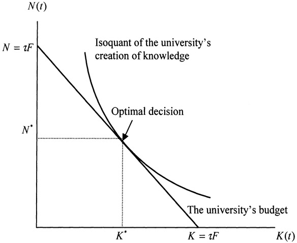
Figure 9.2 The University Optimizes the Use of its Resources
where:
ai≡α(1−τ)α(1−τ)+ˉαrτ, ar≡ˉαrτα(1−τ)+ˉαrτ, ˉβ≡1β(1−τ)+ˉβrτ
The capital distribution is determined by the tax rate and the total capital stocks. The labor distribution between the two sectors is invariant in time. As we assume a fixed population, we can treat Ni and Nr as parameters.
As:
F(t)=Z(t)mKι(t)αNι(t)β, Y(t)=F(t),
we have:
F=aαiNβiZmKα, ˆY=F+δK=aαiNβiZmKα+δK.
The disposable income is determined as a function of K(t) and Z(t). Using these equations and equations (9.2.2), we can represent dynamics of K(t) and Z(t) as functions of K(t) and Z(t):
˙K(t)=AkZ(t)mK(t)α−(ξ+δkλ)(t),˙Z(t)=AιZ(t)m−ϵιK(t)α+ArZ(t)ϵrK(t)αr−δzZ(t)(9.2.3)
It can be shown that the dynamic system may have either a single equilibrium or two equilibria. When it has two equilibria, the equilibrium with lower levels of K and Z is stable; the other one is unstable. We now demonstrate the case that the system has two equilibria. Since τi and τr are meaningful for ∞ > τi ≥ 0 and ∞ > τr ≥ 0, the ranges of values that Ai and Ar can be specified are also from zero to a large positive number. It is straightforward to show that equilibrium of the system is a solution of:
K=A0Zm/β,Φ(Z)≡AiAα0Zxi+ArAαr0Zxr-δzZ=0,(9.2.4)
where:
A0≡(Akξk)1/β,xi≡m-εi+αmβ-1,x≡εr+αrmβ-1.
We interpret xi and xr respectively as parameters of returns to scales through learning by doing and through research. As in the previous chapter, we say that the system exhibits increasing (decreasing) returns to scale with learning by doing if xi > (<) 0. Similarly, the economic system is said to exhibit increasing (decreasing) returns to scale with research if xr > (<) 0. It is straightforward to show that if the two sectors exhibit increasing returns, the dynamic system has a unique unstable equilibrium; if the two sectors exhibit decreasing returns, the dynamic system has a unique unstable equilibrium. If one sector exhibits increasing returns and the other sector decreasing returns, then it is possible for the system to have two equilibria - one is called poverty traps and the other one prosperity with knowledge. We now identify existence of two equilibria by simulation.
As K = A0Zmtβ gives a unique relation between K and Z, the number of equilibrium is equal to the number of solution of equation, ϕ(Z) = 0. We specify the parameters in the equation as follows:
AiAα0=0.25, ArAar0=0.3, xi=-0.5,xr=0.3.
Computer gives two solutions Z1 = 0.09 and Z2 = 49.01 of ϕ(Z) = 0. The solutions are illustrated in Figure 9.3. The former solution is called poverty traps; the latter is called prosperity with knowledge. We can calculate all the other variables at the two equilibria. We see that the living standards are totally different in the two states.
We now come back to dynamic analysis. By equations (9.2.3), we express growth rates of K(t) and Z(t) as functions of K(t) and Z(t):
gk(t)≡˙K(t)K(t)=Φk(t)-ξk,


Figure 9.3 Poverty Versus Prosperity Generated by the Same System
gz(t)≡˙Z(t)Z(t)=Φi(t)+Φr(t)-δzZ(t),(9.2.5)
where:
Φk(t)≡AkZ(t)mK(t)α-1, Φi(t)≡AiZ(t)m-ϵi−1K(t)α,Φt(t)≡ArZ(t)εr-1K(t)αr, Ak≡λaαiNβi, Ai≡τiaαiNβi,Ar≡τraαrNβrr.
We now examine impact of changes in the tax rate on short-run growth rates. Differentiation of equations (9.2.5) with respect to τ yields:
dgk(t)dτ=-[αˉαr(α(1-τ)+ˉαrτ)(1-τ)+βˉβr(β(1-τ)+ˉβrτ(1−τ)]Φk<0,dgz(t)dτ=(τλZ(t)ϵi+1)dgk(t)dτ+[ααrτ(α(1-τ)+ˉαrτ)τ+ββr(β(1-τ)+ˉβrτ)(1-τ)]Φr(t).(9.2.6)
An increase in the tax rate reduces the growth rate of capital. From the definition of Φk(t) (which accounts for the positive contribution to growth rate of capital accumulation), we see that as K(t) rises, Φk(t) falls. This means that as the economy becomes enriched in capital, Φk(t) becomes small. For a rich economy, change in τ may have weak impact on gk(t). As gk(t) is negative, dgz(t)/dτ may be either negative or positive. In the case that Φk(t) is small and Φr(t) (which accounts for the university's contribution to the growth rate of knowledge) is large, the growth rate of knowledge rises as τ rises. From the definition of Φr(t), we see that Φr(t) rises (falls) as Z(t) rises in the case of εr > (<) 1. Let us limit discussion to the case of εr < 1. As the economy's knowledge is high, Φr(t) becomes small. When both Φk(t) and Φr(t) are small (which occurs when the economy is rich in physical capital and has high level of knowledge stock), the research policy does not have unambiguous impact on Z(t). The government is actually confusing about possible effects of its research policy, at least in the short term. When both Φk(t) and Φr(t) are large (which may take place when the economy is poor but has high level of knowledge), it may harm knowledge growth as well as capital accumulation if the government further strengthens its research policy. We see that how the government's research policy affects the growth rates of K(t) and Z(t) are situation-dependent. It would be difficult for, for instance, Japanese government to find a research policy that speeds up growth rates of knowledge. The situation in Mainland China may be different, at least in the near future as the economy accumulates more capital but the country has little knowledge.
From:
F=aαiNβiZmKα, ˆY=F+δK=aαiNβiZmKα+δK.
the growth rates of the current income and the disposable income are:
gY(t)=mgZ(t)+αgk(t), gˆY(t)=gY(t)Y(t)+gk(t)K(t)ˆY(t).
We thus have:
dgY(t)dτ=mgz(t)dτ+αgk(t)dτ,dgˆY(t)dτ=Y(t)ˆY(t)dgY(t)dτ+K(t)ˆY(t)K(t) dgk (t)dτ
We see that when high levels of capital and knowledge are low in an economy, the growth rates of the current income and the disposable income will be reduced as research policy is strengthened. If the economy is rich in physical capital but poor in knowledge, an increase in the tax rate raises the growth rates of the current and disposable incomes. Nevertheless, when the economy is rich both in physical capital and knowledge, impact of changes in the research policy is ambiguous. In 1990 Zhang provided growth model with learning by doing and research that gives a similar conclusion.9 In 1992 Young also argues that an economy that devotes too many resources to research at the expense of learning by doing may actually slow the long-run rate of growth. We see that this possibility depends crucially on the stage of economic development and learning and research efficiencies.10
9.3 Intermezzo for Multiple Equilibria and Poverty Traps
A key theme in the literature of economic development is poverty traps, which can be perceived as a stable steady with low levels of per capita output and capital stock. This state is called a trap because, if agents attempt to break out of it, then the economy has a tendency to return the low-level steady state. In the early literature of economic development, poverty trap did cause attention of economists who were concerned with economic development of not only the rich but also the poor. In 1952 Nurkse proposed the seemingly banal proposition that countries are poor because they are poor.11 Then he examines what mechanisms will keep them in poverty.12 It is argued that there are possible two processes that prevent low-income from take-off. First, factor growth rates of capital and labor are changed in such a way that they perpetuate poverty. The Malthusian process grows the population faster than improvement in living standard and saving traps make it impossible to rapidly accumulate capital. Partly because of low level of human capital, poor countries tend to have low rates of return in both labor and capital.
Although an extension of the Solow model was said to generate a poverty trap as demonstrated in Section 3.7, we don't interpret that state with low per capita capital as a true trap since the poor state is not stable. Any small chance - not necessary any big push - can drive the economy out of the trap in the extended Solow model. In other words, the extended Solow model shifts the origin (which is an unstable point) in the original Solow model to the trap by making the saving rate an endogenous variable. Poverty traps can also be identified with some models with non-constant saving rates.13 We may illustrate a typical way to generating poverty traps in the OSG model.
Let us consider the growth rate equation for the OSG model gk(t) = λf(k)/ k - (ξk + n). If we assume that the production function is neoclassical, then the average product of capital, f(k)/k, declines with k. Nevertheless, this average product may rise with k in some models with increasing returns due to, for instance, learning by doing or infrastructures. It is possible to generate poverty traps even in the one-sector economy that has an interval of diminishing average product of capital that is followed by a range of rising average product. Figure 9.4 portrays a growth diagram with a λf/k curve and the ξk + n line.
We see that the λf/k curve has the negative slope at low levels of per capita capital, is then followed by a range with a positive slope, and then continuously has the negative slope as k rises. As argued by Barro and Sala-i-Martin,14 the curve may exhibit the assumed pattern with the following reasons. An economy at low levels of development tends to focus on agriculture, which is characterized by diminishing returns to scale. As the economy becomes richer, it typically concentrates more on industry and services. These two sectors may involve ranges of increasing returns due to, for instance, spillovers, learning by doing, division of labor. Eventually, increasing returns would disappear and economy again evolves with diminishing returns. As shown the figure, the system has three equilibria - the λf/k curve crosses the ξk + n line three times. The steady state with the low value of k is stable. This equilibrium constitutes a poverty trap for countries that begin with k between 0 and k*middle. If an economy begins with k > k*middle, then it converges to k*high. An implication of this model is that even big donations from international organizations to poor countries may matter little in helping them from avoiding poverty in the long term. For instance, let us consider a case that a poor country receives donation of a discrete quantity of capital from the World Bank. If the economy is near its low equilibrium and the donation raises k but to a level below k*middle, the economy would enjoy temporary high levels of income and consumption, but it will return back to its poverty state. But according to this model, if donation is sufficiently large, it is possible for the economy to enjoy affluence even in the long term. Obviously, this model cannot explain East Asian miracles - East Asian economies had not received sufficient donations in their initial stages of economic development. These miracles have been sustainable, except capital accumulation, mainly because of heavy and persistent investment in education even during early stages of industrialization.

Figure 9.4 Multiple Equilibria with Poverty Traps
The above model gives another way to escape poverty traps. The way is to strengthen the propensity to own wealth (and/or reduce the population growth rate). As λ rises and ξ falls, the λf/k curve moves upwards and the ξk + n line moves downwards. From Figure 9.4, we see that this will lead to a higher level of k*low. If the propensity to own wealth is increased enough so that k surpasses the value K*middle and then the propensity to own wealth turns back to its initial value, then the economy would not revert back to k*low but evolves towards k*high.
We now come back to the insights from the model proposed in this chapter. We have demonstrated possibility of two equilibria for the same type of economy. Our analytical results show that two seemingly identical regions may follow radically different development paths, one leading to prosperity, the other to stagnation. Taiwan and Mainland China may provide a proper case for this result. Although they had similar backgrounds in terms of cultural heritages, values, and initial human capital, Taiwan and Mainland China had experienced totally different paths of industrialization during the period of 1950-1980 - the former rapidly moved to the high equilibrium, while the latter cycled around the low equilibrium.
Identification of poverty traps in theoretical models has important implications for policy making. When an economy is trapped into stable poverty, one cannot escape the traps by small policy intervention or foreign aids. The economy needs either large short-term policy interventions or large amount of foreign aids to sustain economic progress. Moreover, even large interventions may fail if the society does not learn, for instance, about how to live with inequality, growth, and class mobility. In an evolutional economy, as demonstrated in our example, it is possible that national growth is governed by a path-dependent process such that depending on initial conditions, otherwise identical national economies may remain for long periods of time (if not indefinitely) locked into poverty. We point out that poverty traps do not refer to situations in which it is impossible to escape low incomes. It is generally true that initial conditions matter: a country's average income level in the recent past affects current outcomes but these situations need not generate a poverty trap. Economic development of Taiwan provides a good example for escaping from poverty. Since good and bad outcomes are self-enforcing in an evolutionary economy, it is important to take account of small interventions or chance events since they alter the long-term outcome.
When dynamic economic systems have multiple equilibria, one can find different dynamic processes of how a particular equilibrium actually gets established. One explanation is to emphasize decisive role of history or initial conditions. For instance, according to Max Weber's celebrated analysis of East Asian cultures, Chinese culture is more suitable for industrialization than Japanese culture.15 But the modern economic history showed that Japan was much faster in escaping poverty trap than China. As demonstrated by Zhang, 16 this difference in industrialization was strongly influenced by the initial conditions of the two economies when the West came to enforce East Asia to open their doors. Another process to be trapped into an attractor is by expectations. Big push models like the model of Rosenstein-Rodan emphasize the role of expectations about investment by other firms and self-fulfilling prophecy. The government can push the economy out of the trap by coordinating expectations around high demand and high investment. It is important to note that in an economic model with multiple equilibria, the past as well as expected future can play a decisive role in a nation's development paths. Multiplicity of equilibria also means that cultural, sociological and political factors, which have been treated as trivial factors, may play a decisive role in influencing processes of economic bifurcations from poverty into prosperity, and vice versa. Indeed, the importance of hysteresis in a model of multiple equilibria with increasing returns has been highlighted in works, for instance, on path-dependence in technological development and industrial location in developed economies and in models of unemployment, on expectation-driven dynamics in models of network externalities in technology adoption.
The analytical results from the previous sector can be applied to provide some insights into Rosenstein-Rodan's ideas that simultaneous industrialization of many sectors of the economy can be profitable for them all even when no sector can break even industrializing alone. The idea of a backward economy making a big push into industrialization by coordinating investments across sectors has played an important role in the development of development economics. Rosenstein-Rodan pointed out in 1943 that economic development could be conceived as a massive coordination failure - several investments do not occur simply because other complementary investments are not made, and these latter investments are not forthcoming simply because the former are missing.17 According to Rosenstein-Rodan, if multiple sectors of the economy adopted increasing returns technologies simultaneously, they could each yield income that becomes a source of demand for goods in other sectors, and so expand their markets and make industrialization profitable. This industrializing process can be self-sustained even if no sector could break industrializing alone. This insight became the seed for the development of the big-push theory.18 The big-push theory holds that the same economy must be capable of both the backward pre-industrial and modern industrialized state. Simultaneous investments by all the sectors using the available technology would enable the economy to industrialize, without any exogenous improvement in endowments or technologies.
One might conceive of two equilibria under the very same fundamental conditions, one in which active investment is taking place, with each industry's progress supported and justified by the expansion of other sectors of the system, and another equilibrium characterized by persistent stagnation. In the equilibrium of poverty the inactivity of one industry seeps into another - there is no sufficient force for the economy to jump into another equilibrium point once the economy is trapped into poverty. This argument gives an explanation of why similar economies may behave very differently, depending on the nature of beliefs held by agents in different sectors concerning the actions of each other. In our system, this situation occurs when one sector exhibits increasing returns to scale and the other sector exhibits decreasing returns to scale. Multiple equilibria exists because the interactive effects or externalities across the two sectors. The expansion of one sector may provoke a great demand for the product of the other or speed up the production and increase productivity of the other sector. In an abstract sense, the sector with increasing returns to scale plays the role of leading sectors in the literature of development economics.
In 1989 Murphy et al provided an interpretation of this idea in the context of an imperfectly competitive economy with large fixed costs and aggregate demand spillovers.19 The source of multiplicity of equilibria is pecuniary externalities generated by imperfect competition with large fixed costs. In particular, they interpreted the big push into industrialization as a move from a bad to a good equilibrium. They give three examples: a company adopting increasing returns must be:
- (i) shifting demand toward manufacturing goods, or
- (ii) redistributing demand toward the periods in which other companies sell, or
- (iii) paying part of the cost of the essential infrastructure.
The case of shifting demand toward manufacturing goods raises the demand for other manufactures, making large-scale production in other sectors more attractive. The economic mechanism of case (ii) is similar to that of case (i). In the last case increases in the use of infrastructures will render the provision of these services more viable. In 2000 Ljungquist built a model with increasing returns to educational investment and credit market for investment in human capital.20 In that model, it is assumed that the poor cannot afford to have education and skill formation. In equilibrium a poor country, even when it has the same technology and preferences as the richer countries with which it trades, will remain characterized by a high ratio of unskilled workers in the labor force and a large wage differential between skilled and unskilled workers. It is argued that credit traps can be avoided by mitigating information problems that cause credit market failure.
We now introduce a study on whether a big push with natural resource booms can lead to fast growth. The investigation was conducted by Sachs and Warner,21 based on evidence from seven Latin American countries. According to the big-push idea, an expansion of large demand will expand the size of the market, so that entrepreneurs will find it profitable to incur the fixed costs of industrialization. Any expansion in demand, like a large public spending program, foreign aid, discovery of minerals, or a rise in the world price of a natural resource, can become important catalysts for economic development of poor countries. But Sachs and Warner's empirical study shows that natural resource booms are sometimes accompanied by declining per-capita GDP. They provide some reasons for the observed negative association between natural resource and growth. It is argued that resource booms shifts resources away from sectors of the economy that have positive externalities for growth. It is observed that natural resource abundance countries tended to have a larger service sectors and smaller manufacturing sectors than resource-poor economies. Natural resource abundance may also lead to low accumulation in physical and human capital, corruption, and low efficiency of institution. Indeed, the cross-country studies, as mentioned by Sachs and Warner, show that there is no robust association between natural resource abundance and other growth determinants, such as national saving, national investment or rates of human capital accumulation; but there is an inverse association between natural resource abundance and several measures of institutional quality. It should be noted that Spilimbergo et al. also tested the hypothesis that there is a negative interaction effect between natural resource abundance and trade and conclude that the interaction effect has the opposite sign: openness reduces inequality in resource-abundant countries.22 They found that inequality is positively related to the interaction effect between trade and human capital.
The model proposed in this chapter shows that it is possible to formally address Rosenstein-Rodan's ideas not in the context of an imperfectly competitive economy on a disaggregated level. To escape from a low equilibrium is not necessarily in Rosenstein-Rodan's way; it is possible to industrialize by institutional reforms like Japan and China. It is worthwhile to cite the caution given by Lucas when he was discussing economic miracles in East Asia:23 'But simply advising a society to 'follow the Korean model' is a little like advising an aspiring basketball player to 'follow the Michael Jordan model.' To make use of someone else's successful performance at any task, one needs to be able to break this performance down into its component parts so that one can see what each part contributes to the whole, which aspects of this performance are imitable and, of these, which are worth imitating. One needs, in short, a theory.' Stiglitz argued that it is necessary to go far beyond traditional economic theories and into political science to understand the growth miracle of East Asia:24 'No single policy ensured success, nor did the absence of any single ingredient ensure failure. There was a nexus of policies, varying from country to country, sharing the common themes that we have emphasized: governments intervened actively in the market, but used, complemented, regulated, and indeed created markets, rather than supplanted them. Governments created an environment in which markets could thrive. Governments promoted exports, education, and technology; encouraged cooperation between government and industry and between firms and their workers; and at the same time encouraged competition. The real miracle of East Asia may be political more than economic: Why did governments undertake these policies? Why did politicians or bureaucrats not subvert them for their own self interest? ... The recognition of institutional and individual fallibility rise to a flexibility and responsiveness that, in the end, must lie at the root of sustained success.'
Seeking to understand the divergent economic trajectories of rich and poor nations, Myrdal termed the so-called path processes 'circular causation' (which are sometimes modeled as a dynamical system with multiple absorbing states describing vicious and virtuous cycles of poverty and wealth).25 We show that in an economy where capital and knowledge are two main inputs factors, poverty is a stable but undesirable trap. Societies make efforts to escape from poverty traps. Nevertheless, in our model, the economic state is not locked-in into affluence because such a state is unstable. To stay at high living standard, an economy may have to destroy some of its traditional social or even moral principles to maintain an unstable balanced growth. This issue is too complicated to be explored here.
9.4 Equilibrium of the Growth Model with Knowledge
This section examines equilibrium of the model defined in Section 9.1. Because the expressions are too complicated, we will not explicitly express the dynamics in terms of kj(t) and Z(t). We omit issues related to stability of the system.
First, by ḳj(t) = λjΩj - kj and equation (9.1.5), in steady state we have:
λjΩj = kj,τiFZϵi+τrZϵrKαrrNβrr=δ2Z.(9.4.1)
Substituting λjΩj = kj into equations (9.1.4) yields:
cj=ξjkjλj,sj=kj, j=i,r.(9.4.2)
In equilibrium per capita consumption is proportional to per capita wealth (where the proportional rate is the ratio of the propensity to consume and propensity to own wealth) and the current saving per capita is equal to per capita wealth.
In equilibrium the consumer of group j distributes the total available budget among saving sj, consumption of goods cj, and payment for depreciation δkkj. The budget constraint for consumer of group j is:
cj+sj=ˆyj.
Multiplying cj + sj = ŷj by Nj and adding them, we have:
Σ(cj+sj) Nj=ΣˆyjNj.
The total disposable income is equal to the sum of current income and net wealth (wealth minus the depreciation of physical capital): ŷiNi + ŷrNr = Y + δK. We see that Σ(cj + sj)Nj is equal to Y + δK, i.e.:
Σ(cj+sj)Nj = F+δK,
where we use Y = F. This equation states that the sum of the total consumption, total saving, and net depreciation of physical capital is equal to the sum of the output and wealth.
By the above equations and equations (9.4.2), we get:
δikiNi+δrkrNr=F,
where δj ≡ ξj / λj + δk, j = i, r. Substituting equations (9.4.2) into equations (9.1.3) and then using Ui = Ur, we obtain:
ki=Akr,
where A≡Ar/Al(ξr/λr)ξl(λl/ξl)ξl.
This equation states that in steady state the ratio of wealth between the worker and the scientist is proportionally related to the ratio of amenity levels that the scientist and the worker respectively enjoy. The ratio ki / kr of wealth between the worker and the scientist is proportional to (ξr/λr)ξl(λl/ξl)ξl. As ξj + λj = 1, the term can be considered as a function of λj and λr. In fact:
(ξrλr)ξr(λiξi)ξr=(1-λrλr)1−λr(λi1-λi)1−λr
We depict the function, (ξr/λr)ξi(λi/ξi)ξi, as in Figure 9.5 for 0.2 < λr < 0.9 and 0.2 < λi < 0.9. The figure reveals how the ratio of wealth is dependent on the preference structures associated with professions.


Figure 9.5 The Ratio of Wealth and the Preference Structures
The function is the multiplication of two functions (ξr/λr)ξr and ((λi/ξi)ξi. Since the two functions are similar, we illustrate behavior of (λi/ξi)ξi. We plot the function, (λi/ξi)ξi as Figure 9.6. It achieves its maximum near 0.782. The function is rising in λi and after λi = 0.782 it begins to decline in λi.

Figure 9.6 The Ratio of Wealth and λi
By equation (9.4.1), yj = rkj + wj, and the definitions of Ωj, we have:
(δj-r)kj=wj, j=i, r.(9.4.3)
By equation (9.4.3), ki=Akr and wr=ûwj, we solve:
r = δr-ˆuδiA1-A.(9.4.4)
By equation (9.4.3), we see that it is necessary to require min{δi, δr} > r. For convenience of discussion, we require δi > δr, i.e., λr > λr. The requirement means that the scientist's propensity to own wealth is higher than the worker's propensity to own wealth. By equation (9.4.4) and δi > δr, the requirement min{δr, δr} > r is held if 1 > ûA. If û > 1, then it is necessary to have A < 1. If the scientist is paid highly and enjoys doing research, it may be impossible to maintain a meaningful equilibrium (because of the assumed homogenous population). Because of 1 > ûA, r > 0 is guaranteed if δr/δj > ûA. Summarizing the above discussion, we see that δi > r > 0 are guaranteed if:
1>δrδi>ˆuA.(9.4.5)
In the remainder of this section we are concerned only with the case of λr > λr. We may similarly discuss other possible cases. Under inequalities (9.4.5), we solve r by equation (9.4.4). It is straightforward to see that the rate of interest is decreasing in û.
We now solve the other variables. By δikiNi + δrkrNr = F, ki = Akr and (δi - r)ki = wi in equation (9.4.3), we have:
(δiNi + δrNrA)Wl = (δl-r)F.
Substituting wi in equations (9.1.2) into the above equation yields:
δ1+δrNr/ANiδi-r(1-τ)β=1.
By equation (9.1.7) and Kr = ηK, have Ki = (1 - η)K. By equations (9.1.6) and (9.1.2), and wr = ûwi, we solve:
11-τ-1=βˆuNrNi+αη1-η,
where we use Kr/Kj = η/(1 - η). These two equations contain two variables, τ and Nr/Ni. By solving them, we get:
NrNi=n≡{1+αη/(1-η)}(δ-r)/β-δiδr/A-(δi-r)ˆu,1-τ=11+βnˆu+αη/(1-η)<1.(9.4.6)
Under equation (9.4.5), we have δr / A - (δi - r)û > 0. By equation (9.4.6), we see that for Nr/Ni > 0 to be held it is sufficient to require:
(1+αη1-η)(δi-r)>βδi.
This requirement is guaranteed if we require αδi > r to be held. By equations (9.4.4) and (9.4.5), αδi > r is satisfied if α + βûA > δr/ δi. This inequality and equation (9.4.5) are rewritten as follows:
1>α+βˆuA>δrδi>ˆuA.(9.4.7)
Assumption 9.4.1
In the remainder of this section, we assume equation (9.4.7) to be held.
Under equation (9.4.7) we get positive Nr/Ni and τ by equation (9.4.6). By equation (9.4.6) and Ni + Nr = N, we solve the labor distribution as follows:
Ni = N1+n,Nr=nN1+n.(9.4.8)
By equation (9.1.1) and r = (1 - τ)αF/Ki in equation (9.1.2), we solve K = n0Zmtβ, where we use:
Ki=(1−η)K, n0≡{(1−τ)α/r}1/β Nl1−η.
Substituting F = rKi /α(1 - τ), in equation (9.1.2), Kr = ηK, Ki = (1 - η)K and K = n0Zmtβ into the equilibrium equation for the knowledge accumulation in equation (9.4.1), we obtain the following equation:
Φ(Z)≡Φi(Z)+Φr(Z)-δz=0,(9.4.9)
where:
xl≡mβ-εl-1,xr≡αrmβ+ϵr-1,Φl (Z) = τlNβl{(1-η)n0}αZxi, Φr(Z)=τrNβrr(ηn0)αrZxr.
We show that equation (9.4.9) has meaningful solutions. When xi > 0 and xr > 0, Φ(Z) = 0 has a unique positive solution as Φ′(Z) > 0 for any positive Z, Φ(0) < 0 and Φ′(∞) > 0. Similarly, if xi < 0 and xr < 0, Φ(Z) = 0 has a unique positive solution. In the case of xi > 0 and xr < 0, as Φ′(O) > 0 and Φ′(∞) > 0, we see that Φ(Z) = 0 cannot have a unique solution. On the other hand, as Φ′(Z) = 0 has a unique positive solution, we conclude that Φ(Z) = 0 has two solutions if Φ(Z) = 0 has solutions. We can similarly discuss the case of xi < 0 and xr > 0. Summarizing the above discussion, we have the following proposition.
Proposition 9.4.1
Under Assumption 9.4.1, the system has the following properties:
(1) If xi < 0 and xr < 0, the system has a unique equilibrium; (2) If xi > 0 and xr > 0, the system has a unique equilibrium; and (3) If xi > 0 and xr < 0 (xi < 0 and xr > 0), the system has either two equilibria or no equilibrium. The equilibrium values are determined by the following procedure: Z by equation (9.4.9) → K = n0Zm/β → Kr = ηK → Ki = (1 - η)K → Nj, j = i, r, by equations (9.4.8) → τ by equation (9.4.6) → F by equation (9.1.1) → r and wi by equations (9.1.2) → wr = ûwi → kj by equations (9.4.3) → cj and sj by equations (9.4.2) → yj = rKj + wj → Uj by equations (9.1.3).
Since it is difficult to explicitly provide the stability conditions, we omit the issue. We see that the dynamic system may have either a unique equilibrium or multiple equilibria, depending on the research policy, life style parameters and knowledge utilization efficiency and creativity. From the definitions of the parameters and the above discussion, it can be seen that it is reasonable to accept equation (9.4.7). The conditions are guaranteed if the differences in the amenity levels and propensities between two professions are not large. We will provide an example that satisfies equation (9.4.7) later on. As xj determine the properties of the system, to interpret the above proposition, we need to interpret the parameters xj. In xi = m/β + εi - 1, as m is the population's knowledge utilization efficiency parameter and εi is the measurement of returns to scale in the knowledge accumulation by the production sector, we may interpret xi as the measurement of the production sector's returns to scale in the whole system. We say that the knowledge utilization and creation of the production sector exhibits increasing (decreasing) return to scale in the dynamic system when xi >(<) 0. In xr = αrm/β + εr- 1, the parameter εr describes the impact of knowledge on the knowledge creation and αr measures the effects of capital in helping scientists to discover new knowledge. We say that the knowledge utilization and creation of the university exhibits increasing (decreasing) return to scale in the dynamic system when xr >(<) 0. Proposition 9.2.1 says that if the knowledge utilization and creation of the production sector and the university exhibit decreasing (increasing) return to scale in the system, the system has a unique equilibrium. If the knowledge utilization and creation of the production sector (university) exhibits decreasing return to scale in the system and the university (the production sector) exhibits increasing return to scale, the system has two equilibria.
9.5 The Policy on Scientists’ Payment
We are now concerned with the impact of changes in government's policy on scientists' wage rate on the economic structure. Taking derivatives of equations (9.4.4), (9.4.6) and (9.4.8) with respect to û, we get:
1rAdrdˆu=δr-δi(1-ˆuA)(δr-ˆuδiA)<0, 1NidNidˆu=-11+ndndˆu<0,1NrdNrdˆu=1(1+n)ndndˆu>0,1(1-τ)2βdτdˆu=n+ˆudndˆu<0,(9.5.1)
where:
1ˆudndˆu=δi-r-ˆudr/dˆuδr/A-ˆu(δi-r)-1+αη/(1-η){1+αη/(1-η)}(δi-r)-βδidrdˆu>0.
As the ratio û between the scientists' and the workers' wage rates is increased, the rate r of interest is reduced, some labor force will migrate from the production sector to the university and the tax rate τ is increased. By equation (9.4.9), we get the impact on knowledge as follows:
-Φ′dZdˆu=(1NidNidˆu+αnˆu)Φi+{(βrNr-αrNi)dNrdˆu+αrnˆu}Φr,(9.5.2)
where:
nˆu≡-1(1-τ)βdτdˆu1βrdrdˆu.
As discussed before, Φ′ < 0 in the case of xi < 0 and xr < 0 and Φ′ > 0 in the case of xi > 0 and xr > 0. In the case of xi > 0 and xr < 0 ( xi < 0 and xr > 0), if the system has two equilibria, Φ′ < 0 at the lower equilibrium value of Z and Φ′ > 0 at the higher equilibrium value of Z. We see that Φ′ may be either positive or negative. It can be shown that the sign of nû may be either positive or negative. This implies that the right-hand side of equation (9.5.2) may be either positive or negative.
Since it is difficult to get explicit conclusions, for illustration we specify values of some parameter as follows:
δk=0, η=0.1, α = 0,7,β=0.3,λr=16,λi=17,ˆu=1.2, Ai=1.7Ar.(9.5.3)
We neglect the depreciation of capital, i.e., δk = 0. The condition η = 0.1 means that 10 percent of the total capital stocks is spent on R&D activities. The scientist's propensity λr to hold wealth is higher than the worker's propensity λi to hold wealth; but the difference λr - λi is not great. The scientist's wage rate is higher than that of the worker; the amenity level of doing research is lower than that of working in the production sector. Under equation (9.5.3), we directly check that the requirements (9.4.7) are satisfied. Hence, the dynamic system has meaningful equilibria. Under equation (9.5.3), we calculate:
ξr=56,ξi=67,δr=5, δi=6,A=0.482, r = 3.613,n = 0.345, τ=0.168, Nr=0.256N, Ni=0.734N.(9.5.4)
The tax rate is about 17 percent of the total output. About 74 percent of the labor force is employed by the production sector and about 26 percent of the labor force is employed by the university. By equation (9.5.1), we have:
drdˆu=-2.759,1NidN1dˆu=-1.184,1NrdNrdˆu=3.428,1(1-τ)βd′ιdˆu = 1.876,dndˆu=1.592.
By equation (9.5.2) we calculate:
Φ′dZdˆu=0.715Φi+(0.514αr-3.484βr)Φr.(9.5.5)
It is still difficult to explicitly judge the sign of dZ/dû. For simplicity, we assume 0.514αr - 3.484βr > 0, i.e. αr > 6.665βr. Here, we are only concerned with the following two cases:
- Case I: xi < 0, xr < 0, Φ′ < 0; and
- Case II: xi > 0, xr > 0, Φ′ > 0.
By equation (9.5.5), we conclude that in Case I (II), Z is reduced (increase) as the wage ratio between the scientist and the worker is increased. It can be seen that in the case of αr < 6.665βr, the signs of dZ/dû are ambiguous. Taking derivatives of K = n0Zm/β, Kr = ηK, and Ki = (1 - η)K, we obtain:
1KidKidˆu=1KrdKrdˆu=1KdKdˆu=mβZdZdˆu+1NidNidˆu+nˆu=mβZdZdˆu-0.515,
where we use nû = 0.669. We see that in the case of dZ/ d̂u < 0, the levels of the total capital K and the capital stocks, i; and Kr, employed by the two sectors are increased; in the case of d d̂u > 0, K, i. and Kr may be either increased or reduced.
Taking derivatives of equations (9.1.1), (9.1.2) and wr = ûwi, we get:
1FdFdˆu=αKidKrdˆu+βNidNidˆu+mZdZdˆu=mβZdZdˆu-0.715,1widwidˆu=1FdFdˆu-11−τdτdˆu-1NidNidˆu=mβZdZdˆu-0.095,1wrdwdˆu=1wdwidˆu+1ˆu=mβZdZdˆu+0.739.
In the case of dZ/dû < 0, the output F and the wage rates wi of the worker are reduced. In the case of dZ/dû > 0, wr is increased, F and wi may be either increased or reduced. By cj in equations (9.4.2), yj = δjkj and equation (9.4.3), we obtain:
1cidcidˆu=1yidyidˆu=1kidkidˆu=1δi-rdrdˆu+1widwidˆu=mβZdZdˆu-1.251,1crdcrdˆu=1yrdyrdˆu=1krdkdˆu=1δr-rdrdˆu+1wrdwrdˆu=mβZdZdu-1.251.
Summarizing the above results, we have the following conclusions. We assume equation (9.5.3) to be held and αr > 6.665βr. Then, an increase of the ratio û of wage rates between the scientist and the worker has the following impact on the economic structure: The rate r of interest and the labor force Ni employed by the production sector are reduced, and the number of scientists Nr and the tax rate τ are increased. In the case of xr < 0 and xr < 0 ( xi > 0 and xr > 0 ), the level of knowledge Z is reduced (increased), the total capital stocks K and the capital stocks kj employed by the production sector and the university, the total output F, the wage rate wi, the capital stocks kj, the consumption levels cj and the net incomes yj of per scientist and per worker are reduced (may be either reduced or increased), the wage rate wr may be either reduced or increased (is increased).
We see that it is difficult to generally judge the effects of changes in the research policy on the economic structure. Since an increase in û makes some labor force to move from the production sector to the university, it is reasonable to expect that if the university's research efficiency is not high, the national economy suffers from the increased payment for the scientists.
9.6 The Job Amenities and Economic Structure
We are now concerned with the impact of changes in the professional amenity levels, Ai and Ar, on the economic structure. By equations (9.4.4), (9.5.1) and (9.4.8), we
drdA=(δr-δi)rˆu(1-ˆuA)(δr-ˆuδiA)=-6.837,1NidNidA=-I1+ndndˆu=-3.463,1NrdNrdA=1(1+n)ndndA=10.032,1(1-τ)βdτdˆu=(1-τ)ˆudndˆu=4.65,
where:
dndA=δr/A2-ˆudr/dAδ/A-ˆu(δi-r)n-n+αηn/(1-η){1+η/(1-η)}(δi-r)-βδidrdA=4.658.
By the definition of A, a change in A may be caused by change in propensities and Aj, Here, we assume that an increase in A is caused either by increases in Ar or decreases in Ai. The numerical conclusions in the right-hand sides of the above equations are obtained under equations (9.5.3) and (9.5.4). We assume equations (9.5.3) and (9.5.4) to be held. As the amenity to do science is improved, the rate of interest is reduced, some people immigrate from the production sector to the university and the tax rate τ rises.
Taking derivatives of equation (9.4.9) with respect to A yields:
Φ′dZdˆu=(1NidNidA+αnA)Φi−{(βrNr−αrNi)}dNrdˆu+αrnA}Φr=14.527Φi+(5.123αr−10.038βr)Φr,
where:
nA≡-1(1-τ)βdτdA−1βrdrdA=1.658.
We assume 5.123αr - 10.038βr > 0, i.e., αr > 1.96βr. We conclude that in Case I (II), knowledge Z is reduced (increased) as the job amenity of doing science is increased. By:
K=n0Zm/β, Kr=gK, Ki=(1-g)K,
we obtain:
1KidKidA=1KrdKrdA=1KdKdA=mβZdZdA+1NidNidA+nA=mβZdZdA-1.805.
We see that in the case of dZ/dA < 0, the levels of the total capital K and the capital stocks, Ki and Kr, employed by the two sectors are increased; in the case of dZ/dA > 0, K, Ki and Kr may be either increased or reduced. By equations (9.1.1), (9.1.2) and wr = ûwi, we get:
1FdFdA=αKidKrdA+βNidNidA+mZdZdA=mβZdZdA-2.301,1widwidA=1wrdwrdA=1FdFdA-11−τdτdA-1NidNidA=mβZdZdA-0.235.
In the case of dZ/dA < 0, the output F and the wage rates, wi and wr, of the scientist and the worker are reduced. In the case of dZ/dA > 0, F, wi and wr may be either increased or reduced. By cj in equations (9.4.2), yj = δjkj and equation (9.4.3), we obtain:
1cidcidA=1yidyidA=1kidkidA=1δi-rdrdA+1widwdA=mβZdZdA-3.099,1crdcrdA=1yrdyrdA=1krdkrdA=1δr-rdrdA+1wrdwrdA=mβZdZdA-5.164.
We thus have the following lemma.
Lemma 9.6.1
We assume equation (9.5.3) and αr > 1.96βr to be held. Then, an increase of the amenity level Ar of doing science has the following impact on the economic structure: r and Ni are reduced, and Nr and τ are increased; in the case of xi < 0 and xr < 0 (xi > 0 and xr > 0 ), Z is reduced (increased), K, Kj, F, wj, kj, Cj, yj, j = i, r are reduced (may be either reduced or increased).
It can be seen that in the case of xi < 0 and xr < 0, an increase in the amenity level of doing science will not benefit the society because of the shift of labor force from the production sector to the university. It can be seen that even when dZ/dA is positive, the society's living conditions may not be improved by increasing the amenity level of doing science.
9.7 Knowledge Accumulation and Economic Structure
We now introduce human capital into the two-sector model developed in Section 6.3. The economic structure and the economic variables are the same as in Section 6.3. Let us denote the knowledge stock at time t by Z(t). We specify the following production functions:
Fj(t)=AjZmjKαjjNβjj, αj+βj=1, αj, βj>0
where mj (≥ 0) is sector j's efficiency of knowledge utilization. We thus have:
r = aifiki=αspfsks, w=βifi=βspfs,fj=AjZmjkαjj.(9.7.1)
As full employment of labor and capital is assumed, we have:
Ki(t)+Ks(t)=K(t), Ni(t)+Ns(t)=N(t),
which can be re-written in the form of:
ni(t)ki(t)+ns(t)ks(t)=k(t),ni(t)+ns(t)=1,(9.7.2)
where:
k(t)=K(t)N(t), nj(t)=N(t)N(t), j=i, s.
The current income Y(t) is given by Y(t) = rK + wN = Fi + pFs.
The consumer problem is defined by:
Maximize U(t)=C(t)ξS(t)λ, ξ+λ=1, ξ,λ>0s.t.: p(t)C(t) + S(t) = ˆY(t)≡Y(t)+δK(t).
The optimal solution is:
C(t) = ξˆY(t)p(t),S(t)=λˆY(t).(9.7.3)
Capital accumulates according to:
ˉβr≡βr/(αr+βr)(9.7.4)
As consumption good cannot be saved, we have:
C(t)=Fs(t).(9.7.5)
It is assumed that the knowledge accumulation is through learning by doing. We propose the following equation for knowledge growth:
˙Z(t)=τiFi(t)Z(t)ϵi+τs Fs(t)Z(t)ϵs-δzZ(t),(9.7.6)
in which δz (≥ 0) is the depreciation rate of knowledge, and εj and τj (j = i, s) are parameters. We require τj non-negative. The term, τjFj(t)/Z(t)εj, is sector j's contribution to knowledge accumulation through learning by doing.
First, we have to describe the dynamics in terms of a single variable. Substituting k(t) = K(t) / N(t) into (9.7.4) yields:
˙k(t)=λˆy(t)-k(t)=λy(t)-(1-δλ)k(t),(9.7.7)
where:
ˆγ(t)=ˆY(t)N=y(t)+δk(t), y(t)≡Y(t)N=ni(t)fi(ki)+ns(t)fs(ks).
From equations (9.7.3), we have:
c(t)=ξˆy(t)p(t), s(t)=λˆy(t),
where c(t) ≡ C(t)/N and s(t) = S(t)/N. From these equations and S - δK = Fi and C = Fs, we have:
(9.7.8)
By equations (9.7.1), we have ks(t) = αki(t), where α ≡ αsβi/αiβs.
By ks = αki and βifi = βspfs, we solve:
where m ≡ mi - ms. If αi = αs, then the price is given by p = AiZm/As. In the remainder of this section, we require αi ≠ αs.
Corresponding to equations (9.7.2) and ks(t) = αkj(t), we have:
Corresponding to equation (6.3.4), we have:
where:
It is straightforward to show that for any positive k(t)> 0 and Z(t)> 0, ki(t) is uniquely determined as a function of k(t) and z(t). We denote this function by ki(t)= φ(k(t),Z(t)).By equations (9.7.10) and (9.7.11) and according to the definitions of A and A0, we find:
Hence, for ni(t) to satisfy 1 > ni(t) > 0, it is sufficient to have:
By equations (7.2.7), λŷ = nifi(ki) + δk. Substituting this equation into equation (9.7.7) yields:
where we use equations (9.7.10) and (9.7.11).
We now represent knowledge evolution equation (9.7.6) as a function of k(t) and Z(t). By equations (9.7.10), ks = αki, ki = φ, equation (9.7.6) can be rewritten as:
where:
Lemma 9.7.1
The dynamics of the two-sector growth model with endogenous knowledge follow:
For given values of k(t) and Z(t) at any point of time, the other variables are determined by the following procedure: ki(t) = φ(k, Z) → ks(t) = αki(t) → ni(t) and ns(t) by equations (9.7.10) → r(t), w(t), and fj(t), j = i, s by equations (9.7.1) → p(t) by equation (9.7.9) → Nj(t) = nj(t)N → Kj(t) = kj(t)Nj(t) → Fj(t) = fj(t)Nj(t) → Y(t)= Fi(t)+p(t)Fs(t) → Ŷ(t) = Y(t) + δK(t) → C(t)= ξŶ(t) → S(t) = λŶ(t).
Hence, once we determine k(t) and Z(t), we solve all the variables. It can be shown that the system has may have either a unique or two equilibria. Since the analysis is complicated and we can get few new insights (which are different from what we know about the two-sector model in Chapter 6 and the model in the previous sections), we omit any further examination of the model.
9.8 Economic Growth with Knowledge and Multiple Groups
The production aspects of the economic system under consideration are similar to the OSG model developed in Section 5.1. The output and the rate of interest are denoted respectively by F(t) and r(t). The population is classified into two groups, indexed respectively by group 1 and group 2. The variables Nj, Kj(t), Cj(t), Sj(t) and wj(t) are defined as in Section 5.1. We assume that the labor and capital are always fully employed. The total capital stock K(t) and the total qualified labor force N*(t) are given by:
where and mj (≥ 0) is group j's efficiency of knowledge utilization. The parameters, mj, distinguish the difference in productivity of the two groups.
The production function of the economy is given by F(t) = KαN*β, α + β = 1. The marginal conditions are given by:
The current incomes, Yj, j = 1, 2, are given by Yj = rKj + wjNj. The total current income Y(t) is:
The incomes per capita are given:
where yj ≡ Yj / Nj, kj ≡ Kj / Nj and n ≡ N1/N2. As in Section 5.1, group j's consumption and saving are Cj = ξjŶj and Sj = λjŶj. Group j 's capital accumulation is:
where δj ≡ ξj/λj + δk.
For simplicity, we only take account of learning by doing in the knowledge accumulation. We propose the following possible dynamics of knowledge:
in which τj (≥ 0), δj and δz (> 0) are parameters. Here, we interpret as group j's contribution to the knowledge accumulation through learning by doing. The term F/N* is equal to production scale per unity of the qualified labor force. We assume that the contribution to knowledge creation of group j is positively and linearly related to the group's total production scale N*jF/N*. The parameters εj in measure returns to scale in the knowledge accumulation by group j. We interpret τj as a measurement of knowledge accumulation efficiency of group j.
We have thus built the model with endogenous capital and knowledge and wealth distribution between the two groups. The dynamics consist of equations (9.8.1) and (9.8.2). We now express the dynamics in terms of Kj(t) and Z(t). Using the definition of N*:
we express equations (9.8.1) and (9.8.2) as:
(9.8.3)
This is a three-dimensional dynamic system. We may analyze dynamic properties when the two groups have the same preference structure, i.e., λ1 = λ2. This special case has been examined by Zhang.26 Introduce xj ≡ mj - εj - 1, j = 1, 2. According to Zhang's analysis, the following proposition holds.
Proposition 9.8.1
Assume λ1 = λ2. Then
If x1 < 0 and x2 < 0, the system has a unique stable equilibrium;
If x1 > 0 and x2 > 0, the system has a unique unstable equilibrium;
If x1 > 0 and x2 < 0 (x1 < 0 and x2 > 0 ), the system has either two equilibria or no equilibrium. When the system has two equilibria, the one with low values of K and Z is stable; the other one is unstable.
As the two parameters xj determine the properties of the system, to interpret the above proposition, we only need to interpret the parameters xj. As mj is the knowledge utilization efficiency parameter and εj is returns to scale in the knowledge accumulation, we may interpret mj - εj - 1 as measurement of returns to scale in the whole system. We may thus make the following interpretations of the parameters. We say that the knowledge utilization and creation of group j exhibits increasing (decreasing) return to scale in the dynamic system when xj < (>) 0. We can thus interpret Proposition 9.8.1 as follows: if the knowledge utilization and creation of the two groups exhibit decreasing (increasing) returns to scale in the system, the system has a unique stable (unstable) equilibrium; and if the knowledge utilization and creation of one group exhibits decreasing return to scale in the system and the other one exhibits increasing return to scale, the system has two equilibria. The one with higher values of K and Z is unstable, and the other one is stable.
9.9 On Growth with Endogenous Knowledge
In concluding this chapter, we cite an interesting approach to model growth and technological progress by Kremer in 1993.27 He argued that the hypothesis that growth arises from endogenous knowledge accumulation can be tested. He noted that essentially all models of the endogenous growth of knowledge predict that technological progress is an increasing function of population size. The reason is based on the argument that the larger the population, the more there are to make discoveries, and thus the more rapidly knowledge accumulates. Kremer also observes that over almost all of human history, technological progress has led mainly to increase in population rather than increases in output per person. Only in the past few centuries has the impact of technological change fallen to any substantial degree on output per person. The following simple model by Kremer shows that an endogenous technological progress would be associated with the rise of population.
Before developing our model, we consider a simple version of the Kremer's arguments about interdependence between population and economic growth. First, output is a function of technology, labor, and land:
where L denotes the fixed stock of land. It is assumed that the growth rate of knowledge is proportional to population:
where B is a constant. In this model, the population adjusts so that output per capita equals the subsistence level ȳ at any point of time (an unrealistic hypothesis for industrial economies):
In this model, capital which is a key variable in determining modern economic growth is neglected and the limitation of land keeps population finite.
To solve the model, substituting Y(t) = ȳN(t) from equation (9.9.3) into equation (9.9.1) yields:
The population decreases in the subsistence level of output, increases in technology and the amount of land. Noting that ȳ and L are constant and taking derivatives of equation (9.9.4), we have:
(9.9.5)
where we use equation (9.9.2). As time passes, the population grows; the growth rate is proportional to the population. In this model, the population becomes infinite at t* = α/βBN(0). As approximation, the model is valid as the study period may not be very long.
Kremer tests the model by using population estimates extending back to 1 million B.C. It is confirmed that there is a strongly positive, and approximately linear, relationship between population growth and the level of population. A regression of growth on yields:
(9.9.6)
Equation (9.9.3) tells that the growth rate of population is equal to the growth rate of national product, gN = gY. The relation between the growth rate of population and the population is illustrated in Figure 9.7.
There is a statistically significant association between the population and its growth rate. Differentiating equation (9.9.2) with respect to time results in:
(9.9.7)
The equation tells that technological progress is accelerated as the population is exploding. A main assumption in this model is the Malthusian equation (9.9.3), which has proved invalid for high-tech economies. In our approach, we don't take account of the population dynamics because we are mainly concerned with contemporary knowledge-based economies. When we think of economic history as a dynamic whole, it is necessary to consider different growth forces. We close this chapter by citing what Young observed in 1993:28 'Thus, population growth in the typical log-linear model overcomes the concavity in learning and prevents asymptotic stagnation. In the 600 years following the Sung dynasty, China experienced an enormous increase in its population. Contrary to the prediction of the log-linear learning model, this increase did not prevent technological stagnation. .. .If one views technical change as the steady and never ending serendipitous by-product of production experience, then one is completely at a loss to explain the recurring pattern of technological improvement and stagnation apparent in premodern history.'

Figure 9.7 Economic Growth and the Population
Indeed, a main contribution of growth theory with endogenous knowledge and institutional structures is that endogenous growth theory enables scientists to bridge gaps between theory and various strands of empirical and historical literature. Crafts, for instance, pointed out that endogenous innovation growth theory can be applied to explain why productivity was low in Britain in the early nineteenth century and why the industrial revolution occurred in Britain even though many of macro-inventions on which the revolution was founded were carried out in France.29 According to Crafts, there are three likely gains for economic history from applying growth theory with endogenous knowledge and institutional structures. Firstly, as extensions of traditional neoclassical growth theory, growth theories with endogenous knowledge can take account of scope for divergence and of a much richer variety of influences on growth outcomes. Crafts holds that 'The dangers of a Panglossian view of the past and a selective and restrictive search for evidence in evaluating growth performance should be much reduced for the next generation of cliometricians.' New growth theories are constructed on more realistic hypotheses for explaining technological change. Secondly, new growth theories not only consider institutions and policymaking as one of key factors in economic growth, but also treat these elements as part of socioeconomic evolution in a rigorous way. This makes it possible for researchers to focus attention on detailed characteristics and interdependence of institutional structures and policymaking and rigorously demonstrate why they really matter. New growth theories treat institutional arrangements as an intrinsic part of historical accounts of economic growth. Economic models are now constructed on key arguments of traditional historians, which were previously excluded by assumption or treated at best discursively. Thirdly, Craft points out that 'There can be a strong justification to resume the detailed consideration of the reasons for differences in TFP growth rather than to abandon the idea as old fashioned or simply a reflection of measurement error. Informed by new ideas, better techniques of measuring real output and imaginative investigation of the notion of "social capability", it may be possible to refine and extend the estimates of the growth accounting pioneers.'
In the remainder of this book, we will further demonstrate the significance of treating knowledge and institutional as endogenous variables in socioeconomic evolution.
1 Romer(1990).
2 Young (1993).
3 See Zhang (1990, 1993e, 1993f) and Young (1993).
4 The model in this section is initially proposed in Zhang (1996b). Here, we provide a more refined vision.
5 See, for instance, Banerjee and Newman (1993) on relationships between job amenity and occupational choice.
6 Bresnahan and Trajtenberg (1995).
7 A review on related ideas is given by Helpman (1998).
8 Baumol (1990).
9 Zhang (1990, 1992).
10 Young (1992).
11 Nurkse (1952).
12 See slso Nelson (1956).
13 See Galor and Ryder (1989).
14 See Barro and Sala-i-Martin (1995).
15 See Weber's The Religion of China (Weber, 1951). The book discussed implications of Confucianism and Taoism for industrialization. Weber held that the Chinese culture was more suitable for capitalism than the Japanese culture. But the reality is that Japan was faster than China in industrialization. As argued by Zhang (1998), Weber failed to take proper account of geography and historical conditions in socio-economic evolution.
16 Zhang (1998).
17 Rosenstein-Rodan (1943).
18 A comprehensive literature on the subject is referred to Mookherjee and Ray (2001).
19 Murphy, et al (1989). It is remarked that the endogenous emergence of poverty is explained by the presence of other externalities, such as threshold effects in education (e.g., Azariadis and Drazen, 1990), endogenous fertility decisions (e.g., Becker et al., 1990), coordination failures (e.g., Acemoglu, 1996), external effects associated with human capital investment (e.g., Tamura, 1996b, Eicher and García-Peñalosa, 2001), or redistribution (Ghiglino and Sorger, 2002). We will mention a few other approaches below.
20 Ljungquist (2000).
21 Sachs and Warner (1999).
22 Spilimbergo et al. (1999).
23 Lucas (1993).
24 Stiglitz (1996).
25 See Matsuyama (1995) for a modern interpretation of the idea.
26 See Section 5.4 in Zhang (1999a).
27 Kremer (1993).
28 Young (1993).
29 Crafts (1996).