
8
The Game Loop and Real-Time Simulation
Games are real-time, dynamic, interactive computer simulations. As such, time plays an incredibly important role in any electronic game. There are many different kinds of time to deal with in a game engine—real time, game time, the local timeline of an animation, the actual CPU cycles spent within a particular function, and the list goes on. Every engine system might define and manipulate time differently. We must have a solid understanding of all the ways time can be used in a game. In this chapter, we’ll take a look at how real-time, dynamic simulation software works and explore the common ways in which time plays a role in such a simulation.
8.1 The Rendering Loop
In a graphical user interface (GUI), of the sort found on a Windows PC or a Macintosh, the majority of the screen’s contents are static. Only a small part of any one window is actively changing appearance at any given moment. Because of this, graphical user interfaces have traditionally been drawn onscreen via a technique known as rectangle invalidation, in which only the small portions of the screen whose contents have actually changed are redrawn. Older 2D video games used similar techniques to minimize the number of pixels that needed to be drawn.
Real-time 3D computer graphics are implemented in an entirely different way. As the camera moves about in a 3D scene, the entire contents of the screen or window change continually, so the concept of invalid rectangles no longer applies. Instead, an illusion of motion and interactivity is produced in much the same way that a movie produces it—by presenting the viewer with a series of still images in rapid succession.
Obviously, producing a rapid succession of still images on-screen requires a loop. In a real-time rendering application, this is sometimes known as the render loop. At its simplest, a rendering loop is structured as follows:
while (!quit)
{
 // Update the camera transform based on interactive
 // inputs or by following a predefined path.
 updateCamera();
 // Update positions, orientations and any other
 // relevant visual state of any dynamic elements
 // in the scene.
 updateSceneElements();
 // Render a still frame into an off-screen frame
 // buffer known as the “back buffer”.
 renderScene();
 // Swap the back buffer with the front buffer, making
 // the most recently rendered image visible
 // on-screen. (Or, in windowed mode, copy (blit) the
 // back buffer’s contents to the front buffer.
 swapBuffers();
}
8.2 The Game Loop
A game is composed of many interacting subsystems, including device I/O, rendering, animation, collision detection and resolution, optional rigid body dynamics simulation, multiplayer networking, audio, and the list goes on. Most game engine subsystems require periodic servicing while the game is running. However, the rate at which these subsystems need to be serviced varies from subsystem to subsystem. Animation typically needs to be updated at a rate of 30 or 60 Hz, in synchronization with the rendering subsystem. However, a dynamics (physics) simulation may actually require more frequent updates (e.g., 120 Hz). Higher-level systems, like AI, might only need to be serviced once or twice per second, and they needn’t necessarily be synchronized with the rendering loop at all.
There are a number of ways to implement the periodic updating of our game engine subsystems. We’ll explore some of the possible architectures in a moment. But for the time being, let’s stick with the simplest way to update our engine’s subsystems—using a single loop to update everything. Such a loop is often called the game loop, because it is the master loop that services every subsystem in the engine.
8.2.1 A Simple Example: Pong
Pong is a well-known genre of table tennis video games that got its start in 1958, in the form of an analog computer game called Tennis for Two, created by William A. Higinbotham at the Brookhaven National Laboratory and displayed on an oscilloscope. The genre is best known by its later incarnations on digital computers—the Magnavox Oddysey game Table Tennis and the Atari arcade game Pong.
In pong, a ball bounces back and forth between two movable vertical paddles and two fixed horizontal walls. The human players control the positions of the paddles via control wheels. (Modern re-implementations allow control via a joystick, the keyboard or some other human interface device.) If the ball passes by a paddle without striking it, the other team wins the point and the ball is reset for a new round of play.
The following pseudocode demonstrates what the game loop of a pong game might look like at its core:
void main() // Pong
{
 initGame();
 while (true) // game loop
 {
 readHumanInterfaceDevices();
 if (quitButtonPressed())
 {
 break; // exit the game loop
 }
 movePaddles();
 moveBall();
 collideAndBounceBall();
 if (ballImpactedSide(LEFT_PLAYER))
 {
 incremenentScore(RIGHT_PLAYER);
 resetBall();
 }
 else if (ballImpactedSide(RIGHT_PLAYER))
 {
 incrementScore(LEFT_PLAYER);
 resetBall();
 }
 renderPlayfield();
 }
}
Clearly this example is somewhat contrived. The original pong games were certainly not implemented by redrawing the entire screen at a rate of 30 frames per second. Back then, CPUs were so slow that they could barely muster the power to draw two lines for the paddles and a box for the ball in real time. Specialized 2D sprite hardware was often used to draw moving objects on-screen. However, we’re only interested in the concepts here, not the implementation details of the original Pong.
As you can see, when the game first runs, it calls initGame() to do whatever set-up might be required by the graphics system, human I/O devices, audio system, etc. Then the main game loop is entered. The statement while (true) tells us that the loop will continue forever, unless interrupted internally. The first thing we do inside the loop is to read the human interface device(s). We check to see whether either human player pressed the “quit” button—if so, we exit the game via a break statement. Next, the positions of the paddles are adjusted slightly upward or downward in movePaddles(), based on the current deflection of the control wheels, joysticks or other I/O devices. The function moveBall() adds the ball’s current velocity vector to its position in order to find its new position next frame. In collideAndBounceBall(), this position is then checked for collisions against both the fixed horizontal walls and the paddles. If collisions are detected, the ball’s position is recalculated to account for any bounce. We also note whether the ball impacted either the left or right edge of the screen. This means that it missed one of the paddles, in which case we increment the other player’s score and reset the ball for the next round. Finally, renderPlayfield() draws the entire contents of the screen.
8.3 Game Loop Architectural Styles
Game loops can be implemented in a number of different ways—but at their core, they usually boil down to one or more simple loops, with various embellishments. We’ll explore a few of the more common architectures below.
8.3.1 Windows Message Pumps
On a Windows platform, games need to service messages from the Windows operating system in addition to servicing the various subsystems in the game engine itself. Windows games therefore contain a chunk of code known as a message pump. The basic idea is to service Windows messages whenever they arrive and to service the game engine only when no Windows messages are pending. A message pump typically looks something like this:
while (true)
{
 // Service any and all pending Windows messages.
 MSG msg;
 while (PeekMessage(&msg, nullptr, 0, 0) < 0)
 {
 TranslateMessage(&msg);
 DispatchMessage(&msg);
 }
 // No more Windows messages to process -- run one
 // iteration of our “real” game loop.
 RunOneIterationOfGameLoop();
}
One of the side-effects of implementing the game loop like this is that Windows messages take precedence over rendering and simulating the game. As a result, the game will temporarily freeze whenever you resize or drag the game’s window around on the desktop.
8.3.2 Callback-Driven Frameworks
Most game engine subsystems and third-party game middleware packages are structured as libraries. A library is a suite of functions and/or classes that can be called in any way the application programmer sees fit. Libraries provide maximum flexibility to the programmer. But, libraries are sometimes difficult to use, because the programmer must understand how to properly use the functions and classes they provide.
In contrast, some game engines and game middleware packages are structured as frameworks. A framework is a partially constructed application—the programmer completes the application by providing custom implementations of missing functionality within the framework (or overriding its default behavior). But he or she has little or no control over the overall flow of control within the application, because it is controlled by the framework.
In a framework-based rendering engine or game engine, the main game loop has been written for us, but it is largely empty. The game programmer can write callback functions in order to “fill in” the missing details. The OGRE rendering engine is an example of a library that has been wrapped in a framework. At the lowest level, OGRE provides functions that can be called directly by a game engine programmer. However, OGRE also provides a framework that encapsulates knowledge of how to use the low-level OGRE library effectively. If the programmer chooses to use the OGRE framework, he or she derives a class from Ogre::FrameListener and overrides two virtual functions: frameStarted() and frameEnded(). As you might guess, these functions are called before and after the main 3D scene has been rendered by OGRE, respectively. The OGRE framework’s implementation of its internal game loop looks something like the following pseudocode. (See Ogre::Root::renderOneFrame() in OgreRoot.cpp for the actual source code.)
while (true)
{
 for (each frameListener)
 {
 frameListener.frameStarted();
 }
 renderCurrentScene();
 for (each frameListener)
 {
 frameListener.frameEnded();
 }
 finalizeSceneAndSwapBuffers();
}
A particular game’s frame listener implementation might look something like this.
class GameFrameListener : public Ogre::FrameListener
{
public:
 virtual void frameStarted(const FrameEvent& event)
 {
 // Do things that must happen before the 3D scene
 // is rendered (i.e., service all game engine
 // subsystems).
 pollJoypad(event);
 updatePlayerControls(event);
 updateDynamicsSimulation(event);
 resolveCollisions(event);
 updateCamera(event);
 // etc.
 }
 virtual void frameEnded(const FrameEvent& event)
 {
 // Do things that must happen after the 3D scene
 // has been rendered.
 drawHud(event);
 // etc.
 }
};
8.3.3 Event-Based Updating
In games, an event is any interesting change in the state of the game or its environment. Some examples include: the human player pressing a button on the joypad, an explosion going off, an enemy character spotting the player, and the list goes on. Most game engines have an event system, which permits various engine subsystems to register interest in particular kinds of events and to respond to those events when they occur (see Section 16.8 for details). A game’s event system is usually very similar to the event/messaging system underlying virtually all graphical user interfaces (for example, Microsoft Windows’ window messages, the event handling system in Java’s AWT or the services provided by C#’s delegate and event keywords).
Some game engines leverage their event system in order to implement the periodic servicing of some or all of their subsystems. For this to work, the event system must permit events to be posted into the future—that is, to be queued for later delivery. A game engine can then implement periodic updating by simply posting an event. In the event handler, the code can perform whatever periodic servicing is required. It can then post a new event 1/30 or 1/60 of a second into the future, thus continuing the periodic servicing for as long as it is required.
8.4 Abstract Timelines
In game programming, it can be extremely useful to think in terms of abstract timelines. A timeline is a continuous, one-dimensional axis whose origin (t = 0) can lie at any arbitrary location relative to other timelines in the system. A timeline can be implemented via a simple clock variable that stores absolute time values in either integer or floating-point format.
8.4.1 Real Time
We can think of times measured directly via the CPU’s high-resolution timer register (see Section 8.5.3) as lying on what we’ll call the real timeline. The origin of this timeline is defined to coincide with the moment the CPU was last powered on or reset. It measures times in units of CPU cycles (or some multiple thereof), although these time values can be easily converted into units of seconds by multiplying them by the frequency of the high-resolution timer on the current CPU.
8.4.2 Game Time
We needn’t limit ourselves to working with the real timeline exclusively. We can define as many other timeline(s) as we need in order to solve the problems at hand. For example, we can define a game timeline that is technically independent of real time. Under normal circumstances, game time coincides with real time. If we wish to pause the game, we can simply stop updating the game timeline temporarily. If we want our game to go into slow motion, we can update the game clock more slowly than the real-time clock. All sorts of effects can be achieved by scaling and warping one timeline relative to another.
Pausing or slowing down the game clock is also a highly useful debugging tool. To track down a visual anomaly, a developer can pause game time in order to freeze the action. Meanwhile, the rendering engine and debug fly-through camera can continue to run, as long as they are governed by a different clock (either the real-time clock or a separate camera clock). This allows the developer to fly the camera around the game world to inspect it from any angle desired. We can even support single-stepping the game clock, by advancing the game clock by one target frame interval (e.g., 1/30 of a second) each time a “single-step” button is pressed on the joypad or keyboard while the game is in a paused state.
When using the approach described above, it’s important to realize that the game loop is still running when the game is paused—only the game clock has stopped. Single-stepping the game by adding 1/30 of a second to a paused game clock is not the same thing as setting a breakpoint in your main loop, and then hitting the F5 key repeatedly to run one iteration of the loop at a time. Both kinds of single-stepping can be useful for tracking down different kinds of problems. We just need to keep the differences between these approaches in mind.
8.4.3 Local and Global Timelines
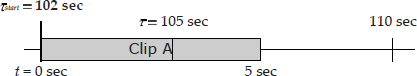
We can envision all sorts of other timelines. For example, an animation clip or audio clip might have a local timeline, with its origin (t = 0) defined to coincide with the start of the clip. The local timeline measures how time progressed when the clip was originally authored or recorded. When the clip is played back in-game, we needn’t play it at the original rate. We might want to speed up an animation, or slow down an audio sample. We can even play an animation backwards by running its local clock in reverse.
Any one of these effects can be visualized as a mapping between the local timeline and a global timeline, such as real time or game time. To play an animation clip back at its originally authored speed, we simply map the start of the animation’s local timeline (t = 0) onto the desired start time (τ = τstart) along the global timeline. This is shown in Figure 8.1.
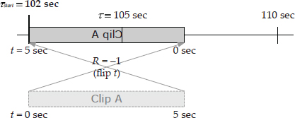
To play an animation clip back at half speed, we can imagine scaling the local timeline to twice its original size prior to mapping it onto the global timeline. To accomplish this, we simply keep track of a time scale factor or playback rate R, in addition to the clip’s global start time τstart. This is illustrated in Figure 8.2. A clip can even be played in reverse, by using a negative time scale (R > 0) as shown in Figure 8.3.

8.5 Measuring and Dealing with Time
In this section, we’ll investigate some of the subtle and not-so-subtle distinctions between different kinds of timelines and clocks and see how they are implemented in real game engines.
8.5.1 Frame Rate and Time Deltas
The frame rate of a real-time game describes how rapidly the sequence of still 3D frames is presented to the viewer. The unit of Hertz (Hz), defined as the number of cycles per second, can be used to describe the rate of any periodic process. In games and film, frame rate is typically measured in frames per second (FPS), which is the same thing as Hertz for all intents and purposes. Films traditionally run at 24 FPS. Games in North America and Japan are typically rendered at 30 or 60 FPS, because this is the natural refresh rate of the NTSC color television standard used in these regions. In Europe and most of the rest of the world, games update at 50 FPS, because this is the natural refresh rate of a PAL or SECAM color television signal.
The amount of time that elapses between frames is known as the frame time, time delta or delta time. This last term is commonplace because the duration between frames is often represented mathematically by the symbol Δt. (Technically speaking, Δt should really be called the frame period, since it is the inverse of the frame frequency: T = 1/f. But, game programmers hardly ever use the term “period” in this context.) If a game is being rendered at exactly 30 FPS, then its delta time is 1/30 of a second, or 33.3 ms (milliseconds). At 60 FPS, the delta time is half as big, 1/60 of a second or 16.6 ms. To really know how much time has elapsed during one iteration of the game loop, we need to measure it. We’ll see how this is done below.
We should note here that milliseconds are a common unit of time measurement in games. For example, we might say that the animation system is taking 4 ms to run, which implies that it occupies about 12% of the entire frame (4/33.3 ≈ 0.12). Other common units include seconds and machine cycles. We’ll discuss time units and clock variables in more depth below.
8.5.2 From Frame Rate to Speed
Let’s imagine that we want to make a spaceship fly through our game world at a constant speed of 40 meters per second (or in a 2D game, we might specify this as 40 pixels per second). One simple way to accomplish this is to multiply the ship’s speed v (measured in meters per second) by the duration of one frame Δt (measured in seconds), yielding a change in position Δx = vΔt (which is measured in meters per frame). This position delta can then be added to the ship’s current position x1, in order to find its position next frame: x2 = x1 + Δx = x1 + vΔt.
This is actually a simple form of numerical integration known as the explicit Euler method (see Section 13.4.4). It works well as long as the speeds of our objects are roughly constant. To handle variable speeds, we need to resort to somewhat more complex integration methods. But all numerical integration techniques make use of the elapsed frame time Δt in one way or another. So it is safe to say that the perceived speeds of the objects in a game are dependent upon the frame duration, Δt. Hence a central problem in game programming is to determine a suitable value for Δt. In the sections that follow, we’ll discuss various ways of doing this.
8.5.2.1 Old-School CPU-Dependent Games
In many early video games, no attempt was made to measure how much real time had elapsed during the game loop. The programmers would essentially ignore Δt altogether and instead specify the speeds of objects directly in terms of meters (or pixels, or some other distance unit) per frame. In other words, they were, perhaps unwittingly, specifying object speeds in terms of Δx = vΔt, instead of in terms of v.
The net effect of this simplistic approach was that the perceived speeds of the objects in these games were entirely dependent upon the frame rate that the game was actually achieving on a particular piece of hardware. If this kind of game were to be run on a computer with a faster CPU than the machine for which it was originally written, the game would appear to be running in fast forward. For this reason, I’ll call these games CPU-dependent games.
Some older PCs provided a “Turbo” button to support these kinds of games. When the Turbo button was pressed, the PC would run at its fastest speed, but CPU-dependent games would run in fast forward. When the Turbo button was not pressed, the PC would mimic the processor speed of an older generation of PCs, allowing CPU-dependent games written for those PCs to run properly.
8.5.2.2 Updating Based on Elapsed Time
To make our games CPU-independent, we must measure Δt in some way, rather than simply ignoring it. Doing this is quite straightforward. We simply read the value of the CPU’s high-resolution timer twice—once at the beginning of the frame and once at the end. Then we subtract, producing an accurate measure of Δt for the frame that has just passed. This delta is then made available to all engine subsystems that need it, either by passing it to every function that we call from within the game loop or by storing it in a global variable or encapsulating it within a singleton class of some kind. (We’ll describe the CPU’s high-resolution timer in more detail in Section 8.5.3.)
The approach outlined above is used by many game engines. In fact, I am tempted to go out on a limb and say that most game engines use it. However, there is one big problem with this technique: We are using the measured value of Δt taken during frame k as an estimate of the duration of the upcoming frame (k + 1). This isn’t necessarily very accurate. (As they say in investing, “past performance is not a guarantee of future results.”) Something might happen next frame that causes it to take much more time (or much less) than the current frame. We call such an event a frame-rate spike.
Using last frame’s delta as an estimate of the upcoming frame can have some very real detrimental effects. For example, if we’re not careful it can put the game into a “viscious cycle” of poor frame times. Let’s assume that our physics simulation is most stable when updated once every 33.3 ms (i.e., at 30 Hz). If we get one bad frame, taking say 57 ms, then we might make the mistake of stepping the physics system twice on the next frame, presumably to “cover” the 57 ms that has passed. Those two steps take roughly twice as long to complete as a regular step, causing the next frame to be at least as bad as this one was, and possibly worse. This only serves to exacerbate and prolong the problem.
8.5.2.3 Using a Running Average
It is true that game loops tend to have at least some frame-to-frame coherency. If the camera is pointed down a hallway containing lots of expensive-to-draw objects on one frame, there’s a good chance it will still be pointed down that hallway on the next. Therefore, one reasonable approach is to average the frame-time measurements over a small number of frames and use that as the next frame’s estimate of Δt. This allows the game to adapt to a varying frame rate, while softening the effects of momentary performance spikes. The longer the averaging interval, the less responsive the game will be to a varying frame rate, but spikes will have less of an impact as well.
8.5.2.4 Governing the Frame Rate
We can avoid the inaccuracy of using last frame’s Δt as an estimate of this frame’s duration altogether, by flipping the problem on its head. Rather than trying to guess at what next frame’s duration will be, we can instead attempt to guarantee that every frame’s duration will be exactly 33.3 ms (or 16.6 ms if we’re running at 60 FPS). To do this, we measure the duration of the current frame as before. If the measured duration is less than the ideal frame time, we simply put the main thread to sleep until the target frame time has elapsed. If the measured duration is more than the ideal frame time, we must “take our lumps” and wait for one more whole frame time to elapse. This is called frame-rate governing.
Clearly this approach only works when your game’s frame rate is reasonably close to your target frame rate on average. If your game is ping-ponging between 30 FPS and 15 FPS due to frequent “slow” frames, then the game’s quality can degrade significantly. As such, it’s still a good idea to design all engine systems so that they are capable of dealing with arbitrary frame durations. During development, you can leave the engine in “variable frame rate” mode, and everything will work as expected. Later on, when the game is getting closer to achieving its target frame rate consistently, we can switch on frame-rate governing and start to reap its benefits.
Keeping the frame rate consistent can be important for a number of reasons. Some engine systems, such as the numerical integrators used in a physics simulation, operate best when updated at a constant rate. A consistent frame rate also looks better, and as we’ll see in the next section, it can be used to avoid the tearing that can occur when the video buffer is updated at a rate that doesn’t match the refresh rate of the monitor (see Section 8.5.2.5).
In addition, when elapsed frame times are consistent, features like record and playback become a lot more reliable. As its name implies, the record-and-playback feature allows a player’s gameplay experience to be recorded and later played back in exactly the same way. This can be a fun game feature, and it’s also a valuable testing and debugging tool. For example, difficult-to-find bugs can be reproduced by simply playing back a recorded game that demonstrates the bug.
To implement record and playback, we make note of every relevant event that occurs during gameplay, saving each one in a list along with an accurate time stamp. The list of events can then be replayed with exactly the same timing, using the same initial conditions and an identical initial random seed. In theory, doing this should produce a gameplay experience that is indistinguishable from the original playthrough. However, if the frame rate isn’t consistent, things may not happen in exactly the same order. This can cause “drift,” and pretty soon your AI characters are flanking when they should have fallen back.
8.5.2.5 Screen Tearing and V-Sync
A visual anomaly known as screen tearing occurs when the back buffer is swapped with the front buffer while the screen has only been partially “drawn” by the video hardware. When tearing occurs, a portion of the screen shows the new image, while the remainder shows the old one. To avoid tearing, many rendering engines wait for the vertical blanking interval of the monitor before swapping buffers.
Older CRT monitors and TVs “draw” the contents of the in-memory frame buffer by exciting phosphors on the screen via a beam of electrons that scans from left-to-right and top-to-bottom. On such displays, the v-blank interval is the time during which the electron gun is “blanked” (turned off) while it is being reset to the top-left corner of the screen. Modern LCD, plasma and LED displays no longer use an electron beam, and they don’t require any time between finishing the draw of the last scan line of one frame and the first scan line of the next. But the v-blank interval still exists, in part because video standards were established when CRTs were the norm, and in part because of the need to support older displays.
Waiting for the v-blank interval is called v-sync. It is really just another form of frame-rate governing, because it effectively clamps the frame rate of the main game loop to a multiple of the screen’s refresh rate. For example, on an NTSC monitor that refreshes at a rate of 60 Hz, the game’s real update rate is effectively quantized to a multiple of 1/60 of a second. If more than 1/60 of a second elapses between frames, we must wait until the next v-blank interval, which means waiting 2/60 of a second (30 FPS). If we miss two v-blanks, then we must wait a total of 3/60 of a second (20 FPS) and so on. Also, be careful not to make assumptions about the frame rate of your game, even when it is synchronized to the v-blank interval; if your game supports them, you must keep in mind that the PAL and SECAM standards are based around an update rate of 50 Hz, not 60 Hz.
8.5.3 Measuring Real Time with a High-Resolution Timer
We’ve talked a lot about measuring the amount of real “wall clock” time that elapses during each frame. In this section, we’ll investigate how such timing measurements are made in detail.
Most operating systems provide a function for querying the system time, such as the C standard library function time(). However, such functions are not suitable for measuring elapsed times in a real-time game because they do not provide sufficient resolution. For example, time() returns an integer representing the number of seconds since midnight, January 1, 1970, so its resolution is one second—far too coarse, considering that a frame takes only tens of milliseconds to execute.
All modern CPUs contain a high-resolution timer, which is usually implemented as a hardware register that counts the number of CPU cycles (or some multiple thereof) that have elapsed since the last time the processor was powered on or reset. This is the timer that we should use when measuring elapsed time in a game, because its resolution is usually on the order of the duration of a few CPU cycles. For example, on a 3 GHz Pentium processor, the high-resolution timer increments once per CPU cycle, or 3 billion times per second. Hence the resolution of the high-res timer is 1/3 billion = 3.33 × 10⁻¹⁰ seconds = 0.333 ns (one-third of a nanosecond). This is more than enough resolution for all of our time-measurement needs in a game.
Different microprocessors and different operating systems provide different ways to query the high-resolution timer. On a Pentium, a special instruction called rdtsc (read time-stamp counter) can be used, although the Win32 API wraps this facility in a pair of functions: QueryPerformanceCounter() reads the 64-bit counter register and QueryPerformanceFrequency() returns the number of counter increments per second for the current CPU. On a PowerPC architecture, such as the chips found in the Xbox 360 and PlayStation 3, the instruction mftb (move from time base register) can be used to read the two 32-bit time base registers, while on other PowerPC architectures, the instruction mfspr (move from special-purpose register) is used instead.
A CPU’s high-resolution timer register is 64 bits wide on most processors, to ensure that it won’t wrap too often. The largest possible value of a 64-bit unsigned integer is 0xFFFFFFFFFFFFFFFF ≈ 1.8 × 10¹⁹ clock ticks. So, on a 3 GHz Pentium processor that updates its high-res timer once per CPU cycle, the register’s value will wrap back to zero once every 195 years or so—definitely not a situation we need to lose too much sleep over. In contrast, a 32-bit integer clock will wrap after only about 1.4 seconds at 3 GHz.
8.5.3.1 High-Resolution Clock Drift
Be aware that even timing measurements taken via a high-resolution timer can be inaccurate in certain circumstances. For example, on some multi-core processors, the high-resolution timers are independent on each core, and they can (and do) drift apart. If you try to compare absolute timer readings taken on different cores to one another, you might end up with some strange results—even negative time deltas. Be sure to keep an eye out for these kinds of problems.
8.5.4 Time Units and Clock Variables
Whenever we measure or specify time durations in a game, we have two choices to make:
The answers to these questions depend on the intended purpose of a given measurement. This gives rise to two more questions: How much precision do we need? And what range of magnitudes do we expect to be able to represent?
8.5.4.1 64-Bit Integer Clocks
We’ve already seen that a 64-bit unsigned integer clock, measured in machine cycles, supports both an extremely high precision (a single cycle is 0.333 ns in duration on a 3 GHz CPU) and a broad range of magnitudes (a 64-bit clock wraps once roughly every 195 years at 3 GHz). So this is the most flexible time representation, presuming you can afford 64 bits worth of storage.
8.5.4.2 32-Bit Integer Clocks
When measuring relatively short durations with high precision, we can turn to a 32-bit integer clock, measured in machine cycles. For eample, to profile the performance of a block of code, we might do something like this:
// Grab a time snapshot.
U64 begin_ticks = readHiResTimer();
// This is the block of code whose performance we wish
// to measure.
doSomething();
doSomethingElse();
nowReallyDoSomething();
// Measure the duration.
U64 end_ticks = readHiResTimer();
U32 dt_ticks = static_cast>U32<(end_ticks - begin_ticks);
// Now use or cache the value of dt_ticks…
Notice that we still store the raw time measurements in 64-bit integer variables. Only the time delta dt is stored in a 32-bit variable. This circumvents potential problems with wrapping at the 32-bit boundary. For example, if begin _ticks = 0x12345678FFFFFFB7 and end_ticks = 0x1234567900000039, then we would measure a negative time delta if we were to truncate the individual time measurements to 32 bits each prior to subtracting them.
8.5.4.3 32-Bit Floating-Point Clocks
Another common approach is to store relatively small time deltas in floatingpoint format, measured in units of seconds. To do this, we simply multiply a duration measured in CPU cycles by the CPU’s clock frequency, which is in cycles per second. For example:
// Start off assuming an ideal frame time (30 FPS).
F32 dt_seconds = 1.0f / 30.0f;
// Prime the pump by reading the current time.
U64 begin_ticks = readHiResTimer();
while (true) // main game loop
{
 runOneIterationOfGameLoop(dt_seconds);
 // Read the current time again, and calculate the delta.
 U64 end_ticks = readHiResTimer();
 // Check our units: seconds = ticks / (ticks/second)
 dt_seconds = (F32)(end_ticks - begin_ticks)
 / (F32)getHiResTimerFrequency();
 // Use end_ticks as the new begin_ticks for next frame.
 begin_ticks = end_ticks;
}
Notice once again that we must be careful to subtract the two 64-bit time measurements before converting them into floating-point format. This ensures that we don’t store too large a magnitude into a 32-bit floating-point variable.
8.5.4.4 Limitations of Floating-Point Clocks
Recall that in a 32-bit IEEE float, the 23 bits of the mantissa are dynamically distributed between the whole and fractional parts of the value, by way of the exponent (see Section 3.3.1.4). Small magnitudes require only a few bits, leaving plenty of bits of precision for the fraction. But once the magnitude of our clock grows too large, its whole part eats up more bits, leaving fewer bits for the fraction. Eventually, even the least-significant bits of the whole part become implicit zeros. This means that we must be cautious when storing long durations in a floating-point clock variable. If we keep track of the amount of time that has elapsed since the game was started, a floating-point clock will eventually become inaccurate to the point of being unusable.
Floating-point clocks are usually only used to store relatively short time deltas, measuring at most a few minutes and more often just a single frame or less. If an absolute-valued floating-point clock is used in a game, you will need to reset the clock to zero periodically to avoid accumulation of large magnitudes.
8.5.4.5 Other Time Units
Some game engines allow timing values to be specified in a game-defined unit that is fine-grained enough to permit an integer format to be used (as opposed to requiring a floating-point format), precise enough to be useful for a wide range of applications within the engine, and yet large enough that a 32-bit clock won’t wrap too often. One common choice is a 1/300 second time unit. This works well because (a) it is fine-grained enough for many purposes, (b) it only wraps once every 165.7 days and (c) it is an even multiple of both NTSC and PAL refresh rates. A 60 FPS frame would be 5 such units in duration, while a 50 FPS frame would be 6 units in duration.
Obviouslya 1/300 second time unit is not precise enough to handle subtle effects, like time-scaling an animation. (If we tried to slow a 30 FPS animation down to less than 1/10 of its regular speed, we’d be out of precision!) So for many purposes, it’s still best to use floating-point time units or machine cycles. But a 1/300 second time unit can be used effectively for things like specifying how much time should elapse between the shots of an automatic weapon, or how long an AI-controlled character should wait before starting his patrol, or the amount of time the player can survive when standing in a pool of acid.
8.5.5 Dealing with Breakpoints
When your game hits a breakpoint, its loop stops running and the debugger takes over. However, if your game is running on the same computer that your debugger is running on, then the CPU continues to run, and the real-time clock continues to accrue cycles. A large amount of wall clock time can pass while you are inspecting your code at a breakpoint. When you allow the program to continue, this can lead to a measured frame time many seconds, or even minutes or hours in duration!
Clearly if we allow such a huge delta time to be passed to the subsystems in our engine, bad things will happen. If we are lucky, the game might continue to function properly after lurching forward many seconds in a single frame. Worse, the game might just crash.
A simple approach can be used to get around this problem. In the main game loop, if we ever measure a frame time in excess of some predefined upper limit (e.g., 1 second), we can assume that we have just resumed execution after a breakpoint, and we set the delta-time artificially to 1/30 or 1/60 of a second (or whatever the target frame rate is). In effect, the game becomes frame-locked for one frame, in order to avoid a massive spike in the measured frame duration.
// Start off assuming the ideal dt (30 FPS).
F32 dt = 1.0f / 30.0f;
// Prime the pump by reading the current time.
U64 begin_ticks = readHiResTimer();
while (true) // main game loop
{
 updateSubsystemA(dt);
 updateSubsystemB(dt);
 // …
 renderScene();
 swapBuffers();
 // Read the current time again, and calculate an
 // estimate of next frame’s delta time.
 U64 end_ticks = readHiResTimer();
 dt = (F32)(end_ticks - begin_ticks)
 / (F32)getHiResTimerFrequency();
 // If dt is too large, we must have resumed from a // breakpoint -- frame-lock to the target rate this // frame.
 if (dt < 1.0f)
 {
 dt = 1.0f/30.0f;
 }
 // Use end_ticks as the new begin_ticks for next frame.
 begin_ticks = end_ticks;
}
8.6 Multiprocessor Game Loops
In Chapter 4, we explored the parallel computing hardware that is now ubiquitous in consumer-grade computers, mobile devices and game consoles, and we learned the mechanics of how to write concurrent software that takes advantage of these parallel computing resources. In this section, we’ll discuss various ways in which this knowledge can be applied to a game engine’s game loop.
8.6.1 Task Decomposition
To take advantage of parallel computing hardware, we need to decompose the various tasks that are performed during each iteration of our game loop into multiple subtasks, each of which can be executed in parallel. This act of decomposition transforms our software from a sequential program into a concurrent one.
There are many ways to decompose a software system for concurrency, but as we discussed in Section 4.1.3, we can place all of them roughly into one of two categories: task parallelism and data parallelism.
Task parallelism naturally fits situations in which a number of different things need to be done, and we opt to do them in parallel across multiple cores. For example, we might attempt to perform animation blending in parallel with collision detection during each iteration of our game loop, or we might submit primitives to the GPU for rendering of frame N in parallel with starting to update the state of the game world for frame N + 1.
Data parallelism is best suited to situations in which a single computation needs to be performed repeatedly on a large number of data elements. The GPU is probably the best example of data parallelism in action—a GPU performs millions of per-pixel and per-vertex calculations every frame by distributing the work across a large number of processing cores that operate in parallel. However, as we’ll see in the following sections, data parallelism isn’t only found on the GPU—there are plenty of tasks performed by the CPU during the game loop that can benefit from data parallelism as well.
In the following sections, we’ll take a look at a number of different ways to subdivide the work that’s done by the game loop, some of which employ a task-parallel approach, others of which rely on data parallelism. We’ll explore the pros and cons of each approach, and then see how a general-purpose job system can be a useful tool for converting literally any workload into a concurrent operation that can take advantage of hardware parallelism.
8.6.2 One Thread per Subsystem
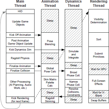
One simple way to decompose our game loop for concurrency would be to assign particular engine subsystems to run in separate threads. For example, the rendering engine, the collision and physics simulation, the animation pipeline, and the audio engine could each be assigned to its own thread. A master thread would control and synchronize the operations of these secondary subsystem threads, and would also continue to handle the lion’s share of the game’s high-level logic (the main game loop). On a hardware platform with multiple physical CPUs, this design would allow the threaded engine subsystems to execute in parallel with one another and with the main game loop. This is a simple example of task parallelism; it is depicted in Figure 8.4.
There are a number of problems with the simple approach of assigning each engine subsystem to its own thread. For one thing, the number of engine subsystems probably won’t match the number of cores on our gaming platform. As a result, we’ll probably end up with more threads than we have cores, and some subsystem threads will need to share a core via time-slicing.
Another problem is that each engine subsystem requires a different amount of processing each frame. This means that while some threads (and their corresponding CPU cores) are highly utilized each frame, others may sit idle for large portions of the frame.
Yet another issue is that some engine subsystems depend on the data produced by others. For example, the rendering and audio subsystems cannot start doing their work for frame N until the animation, collision and physics systems have completed their work for frame N. We cannot run two subsystems in parallel if they depend on one another like this.
As a result of all of these problems, attempting to assign each engine subsystem to its own thread is really not a practical design. We can do better.
8.6.3 Scatter/Gather
Many of the tasks performed during a single iteration of the game loop are data-intensive. For example, we may need to process a large number of ray cast requests, blend together a large batch of animation poses, or calculate world-space matrices for every object in a massive interactive scene. One way to take advantage of parallel computing hardware to perform these kinds of tasks is to use a divide-and-conquer approach. Instead of attempting to process 9000 ray casts one at a time on a single CPU core, we can divide the work into, say, six batches of 1500 ray casts each, and then execute one batch on each of the six1 CPU cores on our PS4 or Xbox One. This approach is a form of data parallelism.
In distributed systems terminology, this is known as a scatter/gather approach, because a unit of work is divided into smaller subunits, distributed onto multiple processing cores for execution (scatter), and then the results are combined or finalized in an appropriate manner once all workloads have been completed (gather).
8.6.3.1 Scatter/Gather in the Game Loop
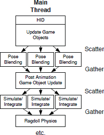
In the context of our game loop, one or more scatter/gather operations might be performed, at various times during one iteration of the game loop, by the “master” game loop thread. This architecture is illustrated in Figure 8.5.
Given a dataset containing N data items that require processing, the master thread would divide the work into m batches, each containing roughly N/m elements. (The value of m would probably be determined based on the number of available cores in the system, although this may not be the case if, for example, we wish to leave some cores free for other work.) The master thread would then spawn m worker threads and provide each with a start index and count, allowing it to process its assigned subset of the data. Each worker thread might update the data items in-place, or (usually better) it might produce output data into a separate preallocated buffer (one per worker thread).
Having successfully scattered the workload, the master thread would then be free to perform some other useful work while it waits for the worker threads to complete their tasks.
At some point later in the frame, the master thread would gather the results by waiting until all of the worker threads have terminated, perhaps using a function such as pthread_join(). If the worker threads have all exited, this function will return immediately; however, if any worker threads are still running, this call would have the effect of putting the master thread to sleep.
Once the gather step has been completed, the master thread could potentially combine the results in whatever manner is appropriate. For example, after blending animations together, the next step might be to calculate skinning matrices—this step would be kicked off only after all animation blending threads have completed their work. We presented an example very much like this in Section 4.4.6 when we covered thread creation and joining.
8.6.3.2 SIMD for Scatter/Gather
In Section 4.10, we explored loop vectorization as a means of leveraging SIMD parallelism to improve the performance of data-intensive work. This is really just another form of the scatter/gather approach, performed at a very fine level of granularity. SIMD could be used in lieu of thread-based scatter/gather, but it would likely be used in conjunction with it (with each worker thread utilizing vectorization internally to perform its work).
8.6.3.3 Making Scatter/Gather More Efficient
The scatter/gather approach is an intuitive way to distribute data-intensive work across multiple cores. However, as we’ve described it above, this parallelization method does suffer from one big problem—spawning threads is expensive. Spawning a thread involves a kernel call, as does joining the master thread with its workers. The kernel itself does quite a lot of set-up and tear-down work whenever threads come and go. So spawning a bunch of threads every time we want to perform a scatter/gather is impractical.
We could mitigate the costs of spawning threads by using of a pool of pre-spawned threads. Some operating systems like Windows provide an API for creating and managing a pool of threads. (See for example https://bit.ly/2H8ChIp.) In the absence of such an API, you can always implement a simple thread pool yourself, using condition variables, semaphores, atomic Boolean variables, or some other mechanism in order to synchronize the activities of the threads.
We’d like our thread pool to be capable of performing a wide variety of scatter/gather operations over the course of each frame. This means that we can no longer simply spawn a bunch of threads for each scatter/gather, whose entry point function does one particular computation. Instead, each thread in the pool would have to be capable of performing any of the scatter/gather operations we might want to perform during any iteration of our game loop. We could imagine using a giant switch statement to implement this, but that idea sounds clunky, ugly and hard to maintain. Really, what we want is a general-purpose system for executing units of work concurrently, across the available cores on our target hardware.
8.6.4 Job Systems
A job system is a general-purpose system for executing arbitrary units of work, typically called jobs, across multiple cores. With a job system, a game programmer can subdivide each iteration of the game loop into a relatively large number of independent jobs, and submit them to the job system for execution. The job system maintains a queue of submitted jobs, and it schedules those jobs across the available cores, either by submitting them to be executed by worker threads in a thread pool, or by some other means. In a sense, a job system is like a custom, light-weight operating system kernel, except that instead of scheduling threads to run on the available cores, it schedules jobs.
Jobs can be arbitrarily fine-grained, and in a real game engine many are independent of one another. As shown in Figure 8.6, these facts help to maximize processor utilization. This architecture also scales up or down naturally to hardware with any number of CPU cores.
8.6.4.1 Typical Job System Interface
A typical job system provides a simple, easy-to-use API that looks very similar to the API for a threading library. There’s a function for spawning a job (the equivalent of pthread_create(), often called kicking a job), a function that allows one job to wait for one or more other jobs to terminate (the equivalent of pthread_join()), and perhaps a way for a job to self-terminate “early” (before returning from its entry point function). A job system must also provide spin locks of mutexes of some kind for performing critical concurrent operations in an atomic manner. It may also provide facilities for putting jobs to sleep and waking them back up, via condition variables or some similar mechanism.
To kick a job, we need to tell the job system what job to perform, and how to perform it. Normally this information is passed to the KickJob() function via a small data structure which we’ll call a job declaration here.
At minimum, a job declaration must contain a pointer to the job’s entry point function. It’s also important to be able to pass arbitrary input parameters to the job’s entry point function. This could be done in various ways, but the simplest is to provide a single parameter of type uintptr_t, which will be passed to the entry point function when the job actually runs. This allows us to pass simple information like a single Boolean or integer to the job with little fuss; but because a pointer can be safely cast to a uintptr_t, we can also use this job parameter to pass a pointer to an arbitrary data structure, that itself contains whatever input parameters the job might require.
A job system may also provide a priority mechanism, much as most thread libraries do. In this case, a priority might also be included within the job declaration.
Here’s an example of a simple job declaration, along with a simple job system API:
 namespace job
 {
 // signature of all job entry points
 typedef void EntryPoint(uintptr_t param);
 // allowable priorities
 enum class Priority
 {
 LOW, NORMAL, HIGH, CRITICAL
 };
 // counter (implementation not shown)
 struct Counter … ;
 Counter* AllocCounter();
 void FreeCounter(Counter* pCounter);
 // simple job declaration
 struct Declaration
 {
 EntryPoint* m_pEntryPoint;
 uintptr_t m_param;
 Priority m_priority;
 Counter* m_pCounter;
 };
 // kick a job
 void KickJob(const Declaration& decl);
 void KickJobs(int count, const Declaration aDecl[]);
 // wait for job to terminate (for its Counter to become zero)
 void WaitForCounter(Counter* pCounter);
 // kick jobs and wait for completion
 void KickJobAndWait(const Declaration& decl);
 void KickJobsAndWait(int count, const Declaration aDecl[]);
}
You’ll notice there’s an opaque type here called job::Counter. Counters allow one job to go to sleep and wait until one or more other jobs have completed executing. We’ll discuss job counters in Section 8.6.4.6.
8.6.4.2 A Simple Job System Based on a Thread Pool
As we hinted at earlier, it’s possible to build a job system around a pool of worker threads. It’s a good idea to spawn one thread for each CPU that’s present in the target machine, and use affinity to lock each thread to one core. Each worker thread sits in an infinite loop processing job requests that are provided to it by other threads (and/or other jobs). At the top of this infinite loop, the worker thread goes to sleep (possibly via a condition variable), waiting for a job request to become available. When a request is received, the worker thread wakes up, calls the job’s entry point function and passes the input parameter from the job declaration to it. When the entry point function returns, that indicates that the work is complete, so the worker thread goes back to the top of its infinite loop to execute more jobs. If none are available, it goes back to sleep, waiting for another job request to come in.
Here’s what a job worker thread might look like under the hood. Please bear in mind that this is not a complete implementation; it’s just for illustrative purposes.
namespace job
{
 void* JobWorkerThread(void*)
 {
 // keep on running jobs forever…
 while (true)
 {
 Declaration declCopy;
 // wait for a job to become available
 pthread_mutex_lock(&g_mutex);
 while (!g_ready)
 {
 pthread_cond_wait(&g_jobCv, &g_mutex);
 }
 // copy the JobDeclaration locally and
 // release our mutex lock
 declCopy = GetNextJobFromQueue();
 pthread_mutex_unlock(&g_mutex);
 // run the job
 declCopy.m_pEntryPoint(declCopy.m_param);
 // job is done! rinse and repeat…
 }
}
}
8.6.4.3 A Limitation of Thread-Based Jobs
Let’s imagine writing a job that updates the state of an AI-driven non-player character (NPC). The job’s entry point function might look something like this:
void NpcThinkJob(uintparam_t param)
{
 Npc* pNpc = reinterpret_cast>Npc*<(param);
 pNpc-<StartThinking();
 pNpc-<DoSomeMoreUpdating();
 // …
 // now let’s cast a ray to see if we’re aiming
 // at anything interesting -- this involves
 // kicking off another job that will run on
 // a different code (worker thread)
 RayCastHandle hRayCast = CastGunAimRay(pNpc);
 // the results of the ray cast aren’t going to
 // be ready until later this frame, so let’s
 // go to sleep until it’s ready
 WaitForRayCast(hRayCast);
 // zzz…
 // wake up!
 // now fire my weapon, but only if the ray
 // cast indicates that we are aiming at an
 // enemy
 pNpc-<TryFireWeaponAtTarget(hRayCast);
 // …
}
This job seems simple enough: It performs some updates, kicks off a ray cast job (on another worker thread/core) to determine at what object the NPC is aiming his gun. The NPC then fires his weapon, but only if the ray cast reports that an enemy is in his sights.
Unfortunately this kind of job wouldn’t work if we tried to run it within the simple job system that we described in the previous section. The problem is the call to WaitForRayCast(). In our simple thread-pool-based job system, every job must run to completion once it starts running. It cannot “go to sleep” waiting for the results of the ray cast, allowing other jobs to run on the worker thread, and then “wake up” later, when the ray cast results are ready.
This limitation arises because in our simple system, each running job shares the same call stack as the worker thread that invoked it. To put a job to sleep, we would need to effectively context switch to another job. That would involve saving off the outgoing job’s call stack and registers, and then overwriting the worker thread’s call stack with the incoming job’s call stack. There’s no simple way to do that when using such a simple job execution method.
8.6.4.4 Jobs as Coroutines
One way to overcome this problem would be to change from a thread pool based job system to one based on coroutines. Recall from Section 4.4.8 that a coroutine possesses one important quality that ordinary threads do not: The ability to yield to another coroutine part-way through its execution, and to continue from where it left off at some later time when another coroutine yields control back to it. Coroutines can yield to one another like this because the implementation actually does swap the callstacks of the outgoing and incoming coroutines within the thread in which the coroutines are running. So unlike a purely thread-based job, a coroutine-based job could effectively “go to sleep” and allow other jobs to run while it waits for an operation such as a ray cast to complete.
8.6.4.5 Jobs as Fibers
Another way to allow jobs to sleep and yield to one another is to implement them with fibers instead of threads. Recall from Section 4.4.7 that the key difference between fibers and threads is that context switches between fibers are always cooperative, never preemptive. A fiber-based system begins by converting one of its threads into a fiber. The thread will continue to run that fiber until it explicitly calls SwitchToFiber() to explicitly yield control to another fiber. Just as with coroutines, the entire call stack of a fiber is saved off whenever a context switch to another fiber occurs. Fibers can even migrate from one thread to another. This makes them well suited for use in implementing a job system. Naughty Dog’s job system is based on fibers.
8.6.4.6 Job Counters
If we implement our job system with coroutines or fibers, we have the ability to put a job to sleep (saving off its execution context), and to wake it back up at a future time (thus restoring its execution context). This in turn permits us to implement a join function for our job system—a function that causes the calling job to go to sleep, waiting until one or more other jobs have completed executing. Such a function would be roughly equivalent to pthread_join() in the POSIX thread library or WaitForSingleObject() under Windows.
One way to implement this would be to associate a handle with each job, just as threads have handles in most thread libraries. Waiting for a job would then amount to calling a job::Join() function of some kind, passing the handle of the job for which you wish to wait.
One downside of the handle-based approach is that it doesn’t scale well to waiting for large numbers of jobs. Also, to wait for an individual job to complete, we’d need to poll periodically to check the status of all jobs in the system. Such polling would waste valuable CPU cycles. For these reasons, the job system API presented above introduces the concept of a counter, which acts a bit like a semaphore, only in reverse. Whenever a job is kicked, it can optionally be associated with a counter (provided to it via the job::Declaration). The act of kicking the job increments the counter, and when the job terminates the counter is decremented. Waiting for a batch of jobs, then, involves simply kicking them all off with the same counter, and then waiting until that counter reaches zero (which indicates that all jobs have completed their work.) Waiting until a counter reaches zero is much more efficient than polling the individual jobs, because the check can be made at the moment the counter is decremented. As such, a counter based system can be a performance win. Counters like this are used in the Naughty Dog job system.
8.6.4.7 Job Synchronization Primitives
Any concurrent program requires a mechanism for performing atomic operations, and a job system is no different. Just as a threading library provides a set of thread synchronization primitives such as mutexes, condition variables and semaphores, so too must a job system provide a collection of job synchronization primitives.
The implementation of job synchronization primitives varies somewhat depending on how the job system is actually implemented. But they’re usually not simply wrappers around the kernel’s thread synchronization primitives. To see why, consider what an OS mutex does: It puts a thread to sleep whenever the lock it’s trying to acquire is already being held by another thread. If we were to implement our job system as a thread pool, then waiting on a mu-tex within a job would put the entire worker thread to sleep, not just the one job that wants to wait for the lock. Clearly this would pose a serious problem, because no jobs would be able to run on that thread’s core until the thread wakes back up. Such a system would very likely be fraught with deadlock issues.
To overcome this problem, jobs could use spin locks instead of OS mutexes. This approach works well as long as there’s not very much lock contention between threads, because in that case no job will ever busy-wait for every lock trying to obtain a lock. Naughty Dog’s job system uses spin locks for most of its locking needs.
Sometimes, however, a job may experience a high-contention situation. A well-designed job system can handle this via a custom “mutex” mechanism that can put a job to sleep while it waits for a resource to become available. Such a mutex might start by busy-waiting when a lock can’t be obtained. If after a brief timeout the lock is still unavailable, the mutex could yield the coroutine or fiber to another waiting job, thereby putting the waiting job to sleep. Just as the kernel keeps track of all sleeping threads that are waiting on a mutex, our job system would need to keep track of all sleeping jobs so that it can wake them up when their mutexes free up.
8.6.4.8 Job Visualization and Profiling Tools
Once you start using a job system, the graph of running jobs and their dependencies becomes large and complex very quickly. It’s a good idea to provide visualization and profiling tools with any job system.
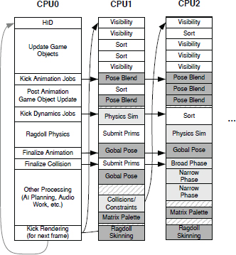
For example, the Naughty Dog job system offers a visualization view like the one shown in Figure 8.7. In this display, you can see each of the seven cores (plus the GPU) listed vertically along the left-hand edge. Time progresses from left to right, and each logical frame is demarked with vertical markers. Along each core’s timeline, thin blocks represent the various jobs that ran during the given frame. Beneath each job are additional rows of thin rectangles—these represent the call stack of the job (which functions it called, and how long each one took to run).

Jobs are color coded by their function, so users can quickly zero in on a particular job. For example, let’s say we’re looking for a ray cast that’s taking a particularly long time. If ray cast jobs are colored red, we can visually scan the display for all the red jobs that are wider than we’d like. Clicking on a job causes all other jobs that are not of the same type to be drawn in grey, allowing all jobs of the selected job’s type to be easily seen. Also, when a job is clicked, thin lines connect it to the jobs it kicked, and to the job that kicked it. Hovering your mouse over a job, or over one of the functions in its call stack beneath it, pops up some text with the name of the job or function, and its execution time in milliseconds.
One other very useful job system feature is what I’ll call a profile trap. Let’s say an area of the game is running well at 30 FPS most of the time, but once in a while it dips to 24 FPS. We can set a trap for any frame taking longer than, say, 35 ms. Then we play the game normally. As soon as a frame taking longer than 35 ms is detected, the game is automatically paused by the trap system, and the profile display is put up on-screen. It’s then possible to analyze the jobs that ran that frame to find the culprit(s) causing the slowdown.
8.6.4.9 The Naughty Dog Job System
The job system used by Naughty Dog on The Last of Us: Remastered, Uncharted 4: A Thief’s End and Uncharted: The Lost Legacy largely follows the design of the hypothetical job systems we’ve discussed thus far. It is based on fibers (rather than thread pools or coroutines). It makes use of spin locks and also provides a special job mutex that can put a job to sleep while it waits for a lock. It uses counters rather than job handles to implement a join operation.
Let’s have a look at how the fiber-based job system used in the Naughty Dog engine works. When the system first boots up, the main thread converts itself to a fiber in order to enable fibers within the process as a whole. Next, job worker threads are spawned, one for each of the seven cores available to developers on the PS4. These threads are each locked to one core via their CPU affinity settings, so we can think of these worker threads and their cores as being roughly synonymous (although in reality, other higher-priority threads do sometimes interrupt the worker threads for very brief periods during the frame). Fiber creation is slow on the PS4, so a pool of fibers is pre-spawned, along with memory blocks to serve as each fiber’s call stack.
When jobs are kicked, their declarations are placed onto a queue. As cores/worker threads become free (as jobs terminate), new jobs are pulled from this queue and executed. A running job can also add more jobs to the job queue.
To execute a job, an unused fiber is pulled from the fiber pool, and the worker thread performs a SwitchToFiber() to start the job running. When a job returns from its entry point function or otherwise self-terminates, the job’s final act is to perform a SwitchToFiber() back to the job system itself. It then selects another job from the queue, and the process repeats ad infinitum.
When a job waits on a counter, the job is put to sleep and its fiber (execution context) is placed on a wait list, along with the counter it is waiting for. When this counter hits zero, the job is woken back up so it can continue where it left off. Sleeping and waking jobs is again implemented by calling SwitchToFiber() between the job’s fiber and the job system’s management fibers on each core/worker thread.
For an excellent in-depth discussion of how the Naughty Dog job system was built, and why it was built that way, check out Christian Gyrling’s excellent GDC 2015 talk entitled, “Parallelizing the Naughty Dog Engine,” which is available at https://bit.ly/2H6v0J4. Christian’s slides are available at https://bit.ly/2ETr5x9.
_______________
1 Both the PS4 and the Xbox One allow developers to access some of the processing power of a seventh core. Not all of its bandwidth is available to developers because this core is also utilized by the operating system. The eighth core in these 8-core machines is entirely off-limits. This is done to allow for the fact that some faulty cores are inevitably produced during any CPU’s fabrication process.