3.1.1.1 Classes and Objects

A class is a collection of attributes (data) and behaviors (code) that together form a useful, meaningful whole. A class is a specification describing how individual instances of the class, known as objects, should be constructed. For example, your pet Rover is an instance of the class “dog.” Thus, there is a one-to-many relationship between a class and its instances.

3.1.1.2 Encapsulation

Encapsulation means that an object presents only a limited interface to the outside world; the object’s internal state and implementation details are kept hidden. Encapsulation simplifies life for the user of the class, because he or she need only understand the class’ limited interface, not the potentially intricate details of its implementation. It also allows the programmer who wrote the class to ensure that its instances are always in a logically consistent state.

3.1.1.3 Inheritance

Inheritance allows new classes to be defined as extensions to preexisting classes. The new class modifies or extends the data, interface and/or behavior of the existing class. If class Child extends class Parent, we say that Child inherits from or is derived from Parent. In this relationship, the class Parent is known as the base class or superclass, and the class Child is the derived class or subclass. Clearly, inheritance leads to hierarchical (tree-structured) relationships between classes.

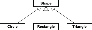
Inheritance creates an “is-a” relationship between classes. For example, a circle is a type of shape. So, if we were writing a 2D drawing application, it would probably make sense to derive our Circle class from a base class called Shape.

We can draw diagrams of class hierarchies using the conventions defined by the Unified Modeling Language (UML). In this notation, a rectangle represents a class, and an arrow with a hollow triangular head represents inheritance. The inheritance arrow points from child class to parent. See Figure 3.1 for an example of a simple class hierarchy represented as a UML static class diagram.

Multiple Inheritance

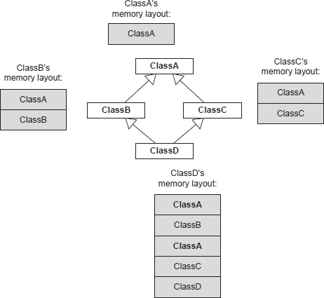
Some languages support multiple inheritance (MI), meaning that a class can have more than one parent class. In theory MI can be quite elegant, but in practice this kind of design usually gives rise to a lot of confusion and technical difficulties (see http://en.wikipedia.org/wiki/Multiple_inheritance). This is because multiple inheritance transforms a simple tree of classes into a potentially complex graph. A class graph can have all sorts of problems that never plague a simple tree—for example, the deadly diamond (http://en.wikipedia.org/wiki/Diamond_problem), in which a derived class ends up containing two copies of a grandparent base class (see Figure 3.2). (In C++, virtual inheritance allows one to avoid this doubling of the grandparent’s data.) Multiple inheritance also complicates casting, because the actual address of a pointer may change depending on which base class it is cast to. This happens because of the presence of multiple vtable pointers within the object.

Most C++ software developers avoid multiple inheritance completely or only permit it in a limited form. A common rule of thumb is to allow only simple, parentless classes to be multiply inherited into an otherwise strictly single-inheritance hierarchy. Such classes are sometimes called mix-in classes because they can be used to introduce new functionality at arbitrary points in a class tree. See Figure 3.3 for a somewhat contrived example of a mix-in class.

3.1.1.4 Polymorphism

Polymorphism is a language feature that allows a collection of objects of different types to be manipulated through a single common interface. The common interface makes a heterogeneous collection of objects appear to be homogeneous, from the point of view of the code using the interface.

For example, a 2D painting program might be given a list of various shapes to draw on-screen. One way to draw this heterogeneous collection of shapes is to use a switch statement to perform different drawing commands for each distinct type of shape.

void drawShapes(std::list<Shape*>& shapes)
{
 std::list<Shape*>::iterator pShape = shapes.begin();
 std::list<Shape*>::iterator pEnd = shapes.end();
 for (; pShape != pEnd; pShape++)
 {
  switch (pShape->mType)
  {
  case CIRCLE:
   // draw shape as a circle
   break;
  case RECTANGLE:
   // draw shape as a rectangle
   break;
  case TRIANGLE:
   // draw shape as a triangle
break;
 //…
}
}
}

The problem with this approach is that the drawShapes() function needs to “know” about all of the kinds of shapes that can be drawn. This is fine in a simple example, but as our code grows in size and complexity, it can become difficult to add new types of shapes to the system. Whenever a new shape type is added, one must find every place in the code base where knowledge of the set of shape types is embedded—like this switch statement—and add a case to handle the new type.

The solution is to insulate the majority of our code from any knowledge of the types of objects with which it might be dealing. To accomplish this, we can define classes for each of the types of shapes we wish to support. All of these classes would inherit from the common base class Shape. A virtual function—the C++ language’s primary polymorphism mechanism—would be defined called Draw(), and each distinct shape class would implement this function in a different way. Without “knowing” what specific types of shapes it has been given, the drawing function can now simply call each shape’s Draw() function in turn.

struct Shape
{
virtual void Draw() = 0; // pure virtual function
virtual ∼Shape() {} // ensure derived dtors are virtual
};
struct Circle : public Shape
{
 virtual void Draw()
 {
  // draw shape as a circle
 }
};
struct Rectangle : public Shape
{
 virtual void Draw()
{
  // draw shape as a rectangle
}
};
struct Triangle : public Shape
{
 virtual void Draw()
{
  // draw shape as a triangle
}
};
 void drawShapes(std::list<Shape*>& shapes)
{
 std::list<Shape*>::iterator pShape = shapes.begin();
 std::list<Shape*>::iterator pEnd = shapes.end();
 for (; pShape != pEnd; pShape++)
 {
pShape->Draw(); // call virtual function
}
}

3.1.1.5 Composition and Aggregation

Composition is the practice of using a group of interacting objects to accomplish a high-level task. Composition creates a “has-a” or “uses-a” relationship between classes. (Technically speaking, the “has-a” relationship is called composition, while the “uses-a” relationship is called aggregation.) For example, a spaceship has an engine, which in turn has a fuel tank. Composition/aggregation usually results in the individual classes being simpler and more focused. Inexperienced object-oriented programmers often rely too heavily on inheritance and tend to underutilize aggregation and composition.

As an example, imagine that we are designing a graphical user interface for our game’s front end. We have a class Window that represents any rectangular GUI element. We also have a class called Rectangle that encapsulates the mathematical concept of a rectangle. A naïve programmer might derive the Window class from the Rectangle class (using an “is-a” relationship). But in a more flexible and well-encapsulated design, the Window class would refer to or contain a Rectangle (employing a “has-a” or “uses-a” relationship). This makes both classes simpler and more focused and allows the classes to be more easily tested, debugged and reused.

3.1.1.6 Design Patterns

When the same type of problem arises over and over, and many different programmers employ a very similar solution to that problem, we say that a design pattern has arisen. In object-oriented programming, a number of common design patterns have been identified and described by various authors. The most well-known book on this topic is probably the “Gang of Four” book [19].

Here are a few examples of common general-purpose design patterns.

The game industry has its own set of design patterns for addressing problems in every realm from rendering to collision to animation to audio. In a sense, this book is all about the high-level design patterns prevalent in modern 3D game engine design.

class AllocJanitor
{
public:
 explicit AllocJanitor(mem::Context context)
 {
  mem::PushAllocator(context);
 }
 ∼AllocJanitor()
 {
  mem::PopAllocator();
 }
};

void f()
{
 // do some work…
 // allocate temp buffers from single-frame allocator
 {
  AllocJanitor janitor(mem::Context::kSingleFrame);
  U8* pByteBuffer = new U8[SIZE];
  float* pFloatBuffer = new float[SIZE];
   // use buffers…
   // (NOTE: no need to free the memory because we // used a single-frame allocator)
   } // janitor pops allocator when it drops out of scope
  // do more work…
}

3.1.2.1 Further Reading

There are plenty of great online resources and books that describe the features of C++11, C++14 and C++17 in detail, so we won’t attempt to cover them here. Here are a few useful references:

3.1.2.2 Which Language Features to Use?

As you read about all the cool new features being added to C++, it’s tempting to think that you need to use all of these features in your engine or game. However, just because a feature exists doesn’t mean your team needs to immediately start making use of it.

At Naughty Dog, we tend to take a conservative approach to adopting new language features into our codebase. As part of our studio’s coding standards, we have a list of those C++ language features that are approved for use in our runtime code, and another somewhat more liberal list of language features that are allowed in our offline tools code. There are a number of reasons for this cautious approach, which I’ll outline in the following sections.

3.2.2.1 Handling Player Errors

When the “user” is the person playing your game, errors should obviously be handled within the context of gameplay. For example, if the player attempts to reload a weapon when no ammo is available, an audio cue and/or an animation can indicate this problem to the player without taking him or her “out of the game.”

3.2.2.2 Handling Developer Errors

When the “user” is someone who is making the game, such as an artist, animator or game designer, errors may be caused by an invalid asset of some sort. For example, an animation might be associated with the wrong skeleton, or a texture might be the wrong size, or an audio file might have been sampled at an unsupported sample rate. For these kinds of developer errors, there are two competing camps of thought.

On the one hand, it seems important to prevent bad game assets from persisting for too long. A game typically contains literally thousands of assets, and a problem asset might get “lost,” in which case one risks the possibility of the bad asset surviving all the way into the final shipping game. If one takes this point of view to an extreme, then the best way to handle bad game assets is to prevent the entire game from running whenever even a single problematic asset is encountered. This is certainly a strong incentive for the developer who created the invalid asset to remove or fix it immediately.

On the other hand, game development is a messy and iterative process, and generating “perfect” assets the first time around is rare indeed. By this line of thought, a game engine should be robust to almost any kind of problem imaginable, so that work can continue even in the face of totally invalid game asset data. But this too is not ideal, because the game engine would become bloated with error-catching and error-handling code that won’t be needed once the development pace settles down and the game ships. And the probability of shipping the product with “bad” assets becomes too high.

In my experience, the best approach is to find a middle ground between these two extremes. When a developer error occurs, I like to make the error obvious and then allow the team to continue to work in the presence of the problem. It is extremely costly to prevent all the other developers on the team from working, just because one developer tried to add an invalid asset to the game. A game studio pays its employees well, and when multiple team members experience downtime, the costs are multiplied by the number of people who are prevented from working. Of course, we should only handle errors in this way when it is practical to do so, without spending inordinate amounts of engineering time, or bloating the code.

As an example, let’s suppose that a particular mesh cannot be loaded. In my view, it’s best to draw a big red box in the game world at the places that mesh would have been located, perhaps with a text string hovering over each one that reads, “Mesh blah-dee-blah failed to load.” This is superior to printing an easy-to-miss message to an error log. And it’s far better than just crashing the game, because then no one will be able to work until that one mesh reference has been repaired. Of course, for particularly egregious problems it’s fine to just spew an error message and crash. There’s no silver bullet for all kinds of problems, and your judgment about what type of error handling approach to apply to a given situation will improve with experience.

3.2.2.3 Handling Programmer Errors

The best way to detect and handle programmer errors (a.k.a. bugs) is often to embed error-checking code into your source code and arrange for failed error checks to halt the program. Such a mechanism is known as an assertion system; we’ll investigate assertions in detail in Section 3.2.3.3. Of course, as we said above, one programmer’s user error is another programmer’s bug; hence, assertions are not always the right way to handle every programmer error. Making a judicious choice between an assertion and a more graceful error-handling technique is a skill that one develops over time.

3.2.3.1 Error Return Codes

A common approach to handling errors is to return some kind of failure code from the function in which the problem is first detected. This could be a Boolean value indicating success or failure, or it could be an “impossible” value, one that is outside the range of normally returned results. For example, a function that returns a positive integer or floating-point value could return a negative value to indicate that an error occurred. Even better than a Boolean or an “impossible” return value, the function could be designed to return an enumerated value to indicate success or failure. This clearly separates the error code from the output(s) of the function, and the exact nature of the problem can be indicated on failure (e.g., enum Error {kSuccess, kAssetNotFound, kInvalidRange, …}).

The calling function should intercept error return codes and act appropriately. It might handle the error immediately. Or, it might work around the problem, complete its own execution and then pass the error code on to whatever function called it.

3.2.3.2 Exceptions

Error return codes are a simple and reliable way to communicate and respond to error conditions. However, error return codes have their drawbacks. Perhaps the biggest problem with error return codes is that the function that detects an error may be totally unrelated to the function that is capable of handling the problem. In the worst-case scenario, a function that is 40 calls deep in the call stack might detect a problem that can only be handled by the top-level game loop, or by main(). In this scenario, every one of the 40 functions on the call stack would need to be written so that it can pass an appropriate error code all the way back up to the top-level error-handling function.

One way to solve this problem is to throw an exception. Exception handling is a very powerful feature of C++. It allows the function that detects a problem to communicate the error to the rest of the code without knowing anything about which function might handle the error. When an exception is thrown, relevant information about the error is placed into a data object of the programmer’s choice known as an exception object. The call stack is then automatically unwound, in search of a calling function that has wrapped its call in a try-catch block. If a try-catch block is found, the exception object is matched against all possible catch clauses, and if a match is found, the corresponding catch’s code block is executed. The destructors of any automatic variables are called as needed during the stack unwinding process.

The ability to separate error detection from error handling in such a clean way is certainly attractive, and exception handling is an excellent choice for some software projects. However, exception handling does add some overhead to the program. The stack frame of any function that contains a try-catch block must be augmented to contain additional information required by the stack unwinding process. Also, if even one function in your program (or a library that your program links with) uses exception handling, your entire program must use exception handling—the compiler can’t know which functions might be above you on the call stack when you throw an exception.

That said, it is possible to “sandbox” a library or libraries that make use of exception handling, in order to avoid your entire game engine having to be written with exceptions enabled. To do this, you would wrap all the API calls into the libraries in question in functions that are implemented in a translation unit that has exception handling enabled. Each of these functions would catch all possible exceptions in a try/catch block and convert them into error return codes. Any code that links with your wrapper library can therefore safely disable exception handling.

Arguably more important than the overhead issue is the fact that exceptions are in some ways no better than goto statements. Joel Spolsky of Microsoft and Fog Creek Software fame argues that exceptions are in fact worse than gotos because they aren’t easily seen in the source code. A function that neither throws nor catches exceptions may nevertheless become involved in the stack-unwinding process, if it finds itself sandwiched between such functions in the call stack. And the unwinding process is itself imperfect: Your software can easily be left in an invalid state unless the programmer considers every possible way that an exception can be thrown, and handles it appropriately. This can make writing robust software difficult. When the possibility for exception throwing exists, pretty much every function in your codebase needs to be robust to the carpet being pulled out from under it and all its local objects destroyed whenever it makes a function call.

Another issue with exception handling is its cost. Although in theory modern exception handling frameworks don’t introduce additional runtime overhead in the error-free case, this is not necessarily true in practice. For example, the code that the compiler adds to your functions for unwinding the call stack when an exception occurs tends to produce an overall increase in code size. This might degrade I-cache performance, or cause the compiler to decide not to inline a function that it otherwise would have.

Clearly there are some pretty strong arguments for turning off exception handling in your game engine altogether. This is the approach employed at Naughty Dog and also on most of the projects I’ve worked on at Electronic Arts and Midway. In his capacity as Engine Director at Insomniac Games, Mike Acton has clearly stated his objection to the use of exception handling in runtime game code on numerous occasions. JPL and NASA also disallow exception handling in their mission-critical embedded software, presumably for the same reasons we tend to avoid it in the game industry. That said, your mileage certainly may vary. There is no perfect tool and no one right way to do anything. When used judiciously, exceptions can make your code easier to write and work with; just be careful out there!

There are many interesting articles on this topic on the web. Here’s one good thread that covers most of the key issues on both sides of the debate:

3.2.3.3 Assertions

An assertion is a line of code that checks an expression. If the expression evaluates to true, nothing happens. But if the expression evaluates to false, the program is stopped, a message is printed and the debugger is invoked if possible.

Assertions check a programmer’s assumptions. They act like land mines for bugs. They check the code when it is first written to ensure that it is functioning properly. They also ensure that the original assumptions continue to hold for long periods of time, even when the code around them is constantly changing and evolving. For example, if a programmer changes code that used to work, but accidentally violates its original assumptions, they’ll hit the land mine. This immediately informs the programmer of the problem and permits him or her to rectify the situation with minimum fuss. Without assertions, bugs have a tendency to “hide out” and manifest themselves later in ways that are difficult and time-consuming to track down. But with assertions embedded in the code, bugs announce themselves the moment they are introduced—which is usually the best moment to fix the problem, while the code changes that caused the problem are fresh in the programmer’s mind. Steve Maguire provides an in-depth discussion of assertions in his must-read book, Writing Solid Code [35].

The cost of the assertion checks can usually be tolerated during development, but stripping out the assertions prior to shipping the game can buy back that little bit of crucial performance if necessary. For this reason assertions are generally implemented in such a way as to allow the checks to be stripped out of the executable in non-debug build configurations. In C, an assert() macro is provided by the standard library header file <assert.h>; in C++, it’s provided by the <cassert> header.

The standard library’s definition of assert() causes it to be defined in debug builds (builds with the DEBUG preprocessor symbol defined) and stripped in non-debug builds (builds with the NDEBUG preprocessor symbol defined). In a game engine, you may want finer-grained control over which build configurations retain assertions, and which configurations strip them out. For example, your game might support more than just a debug and development build configuration—you might also have a shipping build with global optimizations enabled, and perhaps even a PGO build for use by profile-guided optimization tools (see Section 2.2.4). Or you might also want to define different “flavors” of assertions—some that are always retained even in the shipping version of your game, and others that are stripped out of the non-shipping build. For these reasons, let’s take a look at how you can implement your own ASSERT() macro using the C/C++ preprocessor.

#if ASSERTIONS_ENABLED
// define some inline assembly that causes a break
// into the debugger -- this will be different on each
// target CPU
#define debugBreak() asm {int 3}
// check the expression and fail if it is false #define ASSERT(expr) 
  if (expr) {} 
  else 
 { 
  reportAssertionFailure(#expr, 
    __FILE__, __LINE__); 
  debugBreak(); 
}
#else
#define ASSERT(expr) // evaluates to nothing
#endif

// WARNING: NOT A GOOD IDEA!
#define ASSERT(expr) if (!(expr)) debugBreak()
void f()
{
 if (a < 5)
  ASSERT(a >= 0);
 else
  doSomething(a);
}

void f()
{
if (a < 5)
if (!(a >= 0))
debugBreak();
else // oops! bound to the wrong if()!
doSomething(a);
}

struct NeedsToBe128Bytes
{
 U32 m_a;
 F32 m_b;
 // etc.
};
// sadly this doesn’t work…
ASSERT(sizeof(NeedsToBe128Bytes) == 128);

struct NeedsToBe128Bytes
{
 U32 m_a;
 F32 m_b;
// etc.
};
static_assert(sizeof(NeedsToBe128Bytes) == 128,
 “wrong size”);

#define _ASSERT_GLUE(a, b) a ## b
#define ASSERT_GLUE(a, b) _ASSERT_GLUE(a, b)
#define STATIC_ASSERT(expr) 
 enum 
 { 
  ASSERT_GLUE(g_assert_fail_, __LINE__) 
   = 1 / (int)dl(expr)) 
 }
STATIC_ASSERT(sizeof(int) == 4); // should pass
STATIC_ASSERT(sizeof(float) == 1); // should fail

1>test.cpp(48): error C2131: expression did not evaluate to
    a constant
1> test.cpp(48): note: failure was caused by an undefined
   arithmetic operation

#ifdef __cplusplus
 #if __cplusplus >= 201103L
  #define STATIC_ASSERT(expr) 
   static_assert(expr, 
    “static assert failed:” 
    #expr)
 #else
  // declare a template but only define the
  // true case (via specialization)
 template<bool> class TStaticAssert;
 template<> class TStaticAssert<true> {};
 #define STATIC_ASSERT(expr) 
  enum 
 { 
  ASSERT_GLUE(g_assert_fail_, __LINE__) 
   = sizeof(TStaticAssert<!!(expr)>) 
}
#endif
#endif

1>test.cpp(4 8): error C2027: use of undefined type
    ’TStaticAssert<false>’
1>test.cpp(4 8): note: see declaration of
    ’TStaticAssert<false>’

3.3.1.1 Numeric Bases

People think most naturally in base ten, also known as decimal notation. In this notation, ten distinct digits are used (0 through 9), and each digit from right to left represents the next highest power of 10. For example, the number 7803 = (7 × 10³) + (8 × 10²) + (0 × 10¹) + (3 × 10⁰) = 7000 + 800 + 0 + 3.

In computer science, mathematical quantities such as integers and real-valued numbers need to be stored in the computer’s memory. And as we know, computers store numbers in binary format, meaning that only the two digits 0 and 1 are available. We call this a base-two representation, because each digit from right to left represents the next highest power of 2. Computer scientists sometimes use a prefix of “0b” to represent binary numbers. For example, the binary number 0b1101 is equivalent to decimal 13, because 0b1101 = (1 × 2³) + (1 × 2²) + (0 × 2¹) + (1 × 2⁰) = 8 + 4 + 0 + 1 = 13.

Another common notation popular in computing circles is hexadecimal, or base 16. In this notation, the 10 digits 0 through 9 and the six letters A through F are used; the letters A through F replace the decimal values 10 through 15, respectively. A prefix of “0x” is used to denote hex numbers in the C and C++ programming languages. This notation is popular because computers generally store data in groups of 8 bits known as bytes, and since a single hexadecimal digit represents 4 bits exactly, a pair of hex digits represents a byte. For example, the value 0xFF = 0b11111111 = 255 is the largest number that can be stored in 8 bits (1 byte). Each digit in a hexadecimal number, from right to left, represents the next power of 16. So, for example, 0xB052 = (11 × 16³) + (0 × 16²) + (5 × 16¹) + (2 × 16⁰) = (11 × 4096) + (0 × 256) + (5 × 16) + (2 × 1) = 45,138.

3.3.1.2 Signed and Unsigned Integers

In computer science, we use both signed and unsigned integers. Of course, the term “unsigned integer” is actually a bit of a misnomer—in mathematics, the whole numbers or natural numbers range from 0 (or 1) up to positive infinity, while the integers range from negative infinity to positive infinity. Nevertheless, we’ll use computer science lingo in this book and stick with the terms “signed integer” and “unsigned integer.”

Most modern personal computers and game consoles work most easily with integers that are 32 bits or 64 bits wide (although 8- and 16-bit integers are also used a great deal in game programming as well). To represent a 32-bit unsigned integer, we simply encode the value using binary notation (see above). The range of possible values for a 32-bit unsigned integer is 0x00000000 (0) to 0xFFFFFFFF (4,294,967,295).

To represent a signed integer in 32 bits, we need a way to differentiate between positive and negative vales. One simple approach called the sign and magnitude encoding reserves the most significant bit as a sign bit. When this bit is zero, the value is positive, and when it is one, the value is negative. This leaves us 31 bits to represent the magnitude of the value, effectively cutting the range of possible magnitudes in half (but allowing both positive and negative forms of every distinct magnitude, including zero).

Most microprocessors use a slightly more efficient technique for encoding negative integers, called two’s complement notation. This notation has only one representation for the value zero, as opposed to the two representations possible with simple sign bit (positive zero and negative zero). In 32-bit two’s complement notation, the value 0xFFFFFFFF is interpreted to mean −1, and negative values count down from there. Any value with the most significant bit set is considered negative. So values from 0x00000000 (0) to 0x7FFFFFFF (2,147,483,647) represent positive integers, and 0x80000000 (−2,147,483,648) to 0xFFFFFFFF (−1) represent negative integers.

3.3.1.3 Fixed-Point Notation

Integers are great for representing whole numbers, but to represent fractions and irrational numbers we need a different format that expresses the concept of a decimal point.

One early approach taken by computer scientists was to use fixed-point notation. In this notation, one arbitrarily chooses how many bits will be used to represent the whole part of the number, and the rest of the bits are used to represent the fractional part. As we move from left to right (i.e., from the most significant bit to the least significant bit), the magnitude bits represent decreasing powers of two (…, 16, 8, 4, 2, 1), while the fractional bits represent decreasing inverse powers of two (½, ¼, ⅛, $\frac{1}{16}$, …). For example, to store the number −173.25 in 32-bit fixed-point notation with one sign bit, 16 bits for the magnitude and 15 bits for the fraction, we first convert the sign, the whole part and the fractional part into their binary equivalents individually (negative = 0b1, 173 = 0b0000000010101101 and 0.25 = ¼ = 0b010000000000000). Then we pack those values together into a 32-bit integer. The final result is 0x8056A000. This is illustrated in Figure 3.4.

The problem with fixed-point notation is that it constrains both the range of magnitudes that can be represented and the amount of precision we can achieve in the fractional part. Consider a 32-bit fixed-point value with 16 bits for the magnitude, 15 bits for the fraction and a sign bit. This format can only represent magnitudes up to ±65,535, which isn’t particularly large. To overcome this problem, we employ a floating-point representation.

3.3.1.4 Floating-Point Notation

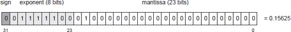
In floating-point notation, the position of the decimal place is arbitrary and is specified with the help of an exponent. A floating-point number is broken into three parts: the mantissa, which contains the relevant digits of the number on both sides of the decimal point, the exponent, which indicates where in that string of digits the decimal point lies, and a sign bit, which of course indicates whether the value is positive or negative. There are all sorts of different ways to lay out these three components in memory, but the most common standard is IEEE-754. It states that a 32-bit floating-point number will be represented with the sign in the most significant bit, followed by 8 bits of exponent and finally 23 bits of mantissa.

The value v represented by a sign bit s, an exponent e and a mantissa m is v = s × 2^(e−127) × (1 + m).

The sign bit s has the value +1 or −1. The exponent e is biased by 127 so that negative exponents can be easily represented. The mantissa begins with an implicit 1 that is not actually stored in memory, and the rest of the bits are interpreted as inverse powers of two. Hence the value represented is really 1 + m, where m is the fractional value stored in the mantissa.

For example, the bit pattern shown in Figure 3.5 represents the value 0.15625, because s = 0 (indicating a positive number), e = 0b01111100 = 124 and m = 0b0100… = 0 × 2⁻¹ + 1 × 2⁻² = ¼. Therefore,

 if (a == b) {…}
 if (a - b == 0.0f) {…}

Portable Sized Types

The built-in primitive data types in C and C++ were designed to be portable and therefore nonspecific. However, in many software engineering endeavors, including game engine programming, it is often important to know exactly how wide a particular variable is.

Before C++11, programmers had to rely on non-portable sized types provided by their compiler. For example, the Visual Studio C/C++ compiler defined the following extended keywords for declaring variables that are an explicit number of bits wide: __int8, __int16, __int32 and __int64. Most other compilers have their own “sized” data types, with similar semantics but slightly different syntax.

Because of these differences between compilers, most game engines achieved source code portability by defining their own custom sized types. For example, at Naughty Dog we use the following sized types:

<cstdint>

The C++11 standard library introduces a set of standardized sized integer types. They are declared in the <cstdint> header, and they include the signed types std::int8_t, std::int16_t, std::int32_t and std::int64_t and the unsigned types std::uint8_t, std::uint16_t, std::uint32_t and std::uint64_t, along with “fast” variants (like the I32F and U32F types we defined at Naughty Dog). These types free the programmer from having to “wrap” compiler-specific types in order to achieve portability. For a complete list of these sized types, see http://en.cppreference.com/w/cpp/types/integer.

OGRE’s Primitive Data Types

OGRE defines a number of sized types of its own. Ogre::uint8, Ogre::uint16 and Ogre::uint32 are the basic unsigned sized integral types.

Ogre::Real defines a real floating-point value. It is usually defined to be 32 bits wide (equivalent to a float), but it can be redefined globally to be 64 bits wide (like a double) by defining the preprocessor macro OGRE_DOUBLE_PRECISION to 1. This ability to change the meaning of Ogre::Real is generally only used if one’s game has a particular requirement for double-precision math, which is rare. Graphics chips (GPUs) always perform their math with 32-bit or 16-bit floats, the CPU/FPU is also usually faster when working in single-precision, and SIMD vector instructions operate on 128-bit registers that contain four 32-bit floats each. Hence, most games tend to stick to single-precision floating-point math.

The data types Ogre::uchar, Ogre::ushort, Ogre::uint and Ogre::ulong are just shorthand notations for C/C++’s unsigned char, unsigned short and unsigned long, respectively. As such, they are no more or less useful than their native C/C++ counterparts.

The types Ogre::Radian and Ogre::Degree are particularly interesting. These classes are wrappers around a simple Ogre::Real value. The primary role of these types is to permit the angular units of hard-coded literal constants to be documented and to provide automatic conversion between the two unit systems. In addition, the type Ogre::Angle represents an angle in the current “default” angle unit. The programmer can define whether the default will be radians or degrees when the OGRE application first starts up.

Perhaps surprisingly, OGRE does not provide a number of sized primitive data types that are commonplace in other game engines. For example, it defines no signed 8-, 16- or 64-bit integral types. If you are writing a game engine on top of OGRE, you will probably find yourself defining these types manually at some point.

3.3.2.1 Multibyte Values and Endianness

Values that are larger than eight bits (one byte) wide are called multibyte quantities. They’re commonplace on any software project that makes use of integers and floating-point values that are 16 bits or wider. For example, the integer value 4660 = 0x1234 is represented by the two bytes 0x12 and 0x34. We call 0x12 the most significant byte and 0x34 the least significant byte. In a 32-bit value, such as 0xABCD1234, the most-significant byte is 0xAB and the least-significant is 0x34. The same concepts apply to 64-bit integers and to 32- and 64-bit floating-point values as well.

Multibyte integers can be stored into memory in one of two ways, and different microprocessors may differ in their choice of storage method (see Figure 3.6).

•Little-endian. If a microprocessor stores the least significant byte of a multibyte value at a lower memory address than the most significant byte, we say that the processor is little-endian. On a little-endian machine, the number 0xABCD1234 would be stored in memory using the consecutive bytes 0x34, 0x12, 0xCD, 0xAB.

•Big-endian. If a microprocessor stores the most significant byte of a multibyte value at a lower memory address than the least significant byte, we say that the processor is big-endian. On a big-endian machine, the number 0xABCD1234 would be stored in memory using the bytes 0xAB, 0xCD, 0x12, 0x34.

 U32 value = 0xABCD1234;
  U8* pBytes = (U8*)&value;

Figure 3.6. Big- and little-endian representations of the value 0xABCD1234.

Most programmers don’t need to think much about endianness. However, when you’re a game programmer, endianness can become a bit of a thorn in your side. This is because games are usually developed on a Windows or Linux machine running an Intel Pentium processor (which is little-endian), but run on a console such as the Wii, Xbox 360 or PlayStation 3—all three of which utilize a variant of the PowerPC processor (which can be configured to use either endianness, but is big-endian by default). Now imagine what happens when you generate a data file for consumption by your game engine on an Intel processor and then try to load that data file into your engine running on a PowerPC processor. Any multibyte value that you wrote out into that data file will be stored in little-endian format. But when the game engine reads the file, it expects all of its data to be in big-endian format. The result? You’ll write 0xABCD1234, but you’ll read 0x3412CDAB, and that’s clearly not what you intended!

There are at least two solutions to this problem.

1.You could write all your data files as text and store all multibyte numbers as sequences of decimal or hexadecimal digits, one character (one byte) per digit. This would be an inefficient use of disk space, but it would work.

2.You can have your tools endian-swap the data prior to writing it into a binary data file. In effect, you make sure that the data file uses the endianness of the target microprocessor (the game console), even if the tools are running on a machine that uses the opposite endianness.

Integer Endian-Swapping

Endian-swapping an integer is not conceptually difficult. You simply start at the most significant byte of the value and swap it with the least significant byte; you continue this process until you reach the halfway point in the value. For example, 0xA7891023 would become 0x231089A7.

The only tricky part is knowing which bytes to swap. Let’s say you’re writing the contents of a C struct or C++ class from memory out to a file. To properly endian-swap this data, you need to keep track of the locations and sizes of each data member in the struct and swap each one appropriately based on its size. For example, the structure

struct Example
{
 U32 m_a;
 U16 m_b;
 U3  m_c;
};

might be written out to a data file as follows:

void writeExampleStruct(Example& ex, Stream& stream)
{
 stream.writeU32(swapU32(ex.m_a));
 stream.writeU16(swapU16(ex.m_b));
 stream.writeU32(swapU32(ex.m_c));
}

and the swap functions might be defined like this:

inline U16 swapU16(U16 value)
{
 return ((value & 0x00FF) << 8)
  | ((value & 0xFF00) >> 8);
}
inline U32 swapU32(U32 value)
{
 return ((value & 0x000000FF) << 24)
  | ((value & 0x0000FF00) << 8)
  | ((value & 0x00FF0000) >> 8)
  | ((value & 0xFF000000) >> 24);
}

You cannot simply cast the Example object into an array of bytes and blindly swap the bytes using a single general-purpose function. We need to know both which data members to swap and how wide each member is, and each data member must be swapped individually.

Some compilers provide built-in endian-swapping macros, freeing you from having to write your own. For example, gcc offers a family of macros named __builtin_bswapXX() for performing 16-, 32- and 64-bit endian swaps. However, such compiler-specific facilities are of course non-portable.

Floating-Point Endian-Swapping

As we’ve seen, an IEEE-754 floating-point value has a detailed internal structure involving some bits for the mantissa, some bits for the exponent and a sign bit. However, you can endian-swap it just as if it were an integer, because bytes are bytes. You merely reinterpret the bit pattern of your float as if it were a std::int32_t, perform the endian swapping operation, and then reinterpret the result as a float again.

You can reinterpret floats as integers by using C++’s reinterpret_cast operator on a pointer to the float, and then dereferencing the type-cast pointer; this is known as type punning. But punning can lead to optimization bugs when strict aliasing is enabled. (See http://www.cocoawithlove.com/2008/04/using-pointers-to-recast-in-c-is-bad.html for an excellent description of this problem.) One alternative that’s guaranteed to be portable is to use a union, as follows:

union U32F32
{
 U32 m_asU32;
 F32 m_asF32;
};
inline F32 swapF32(F32 value)
{
 U32F32 u;
 u.m_asF32 = value;
 // endian-swap as integer
 u.m_asU32 = swapU32(u.m_asU32);
 return u.m_asF32;
}

3.3.3 Kilobytes versus Kibibytes

You’ve probably used metric (SI) units like kilobytes (kB) and megabytes (MB) to describe quantities of memory. However, the use of these units to describe quantities of memory that are measured in powers of two isn’t strictly correct. When a computer programmer speaks of a “kilobyte,” she or he usually means 1024 bytes. But SI units define the prefix “kilo” to mean 10³ or 1000, not 1024.

To resolve this ambiguity, the International Electrotechnical Commission (IEC) in 1998 established a new set of SI-like prefixes for use in computer science. These prefixes are defined in terms of powers of two rather than powers of ten, so that computer engineers can precisely and conveniently specify quantities that are powers of two. In this new system, instead of kilobyte (1000 bytes), we say kibibyte (1024 bytes, abbreviated KiB). And instead of megabyte (1,000,000 bytes), we say mebibyte (1024 × 1024 = 1,048,576 bytes, abbreviated MiB). Table 3.1 summarizes the sizes, prefixes and names of the most commonly used byte quantity units in both the SI and IEC systems. We’ll use IEC units throughout this book.

Table 3.1. Comparison of metric (SI) units and IEC units for describing quantities of bytes.

3.3.4 Declarations, Definitions and Linkage

3.3.4.1 Translation Units Revisited

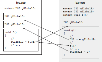
As we saw in Chapter 2, a C or C++ program is comprised of translation units. The compiler translates one .cpp file at a time, and for each one it generates an output file called an object file (.o or .obj). A .cpp file is the smallest unit of translation operated on by the compiler; hence, the name “translation unit.” An object file contains not only the compiled machine code for all of the functions defined in the .cpp file, but also all of its global and static variables. In addition, an object file may contain unresolved references to functions and global variables defined in other .cpp files.

The compiler only operates on one translation unit at a time, so whenever it encounters a reference to an external global variable or function, it must “go on faith” and assume that the entity in question really exists, as shown in Figure 3.7. It is the linker’s job to combine all of the object files into a final executable image. In doing so, the linker reads all of the object files and attempts to resolve all of the unresolved cross-references between them. If it is successful, an executable image is generated containing all of the functions, global variables and static variables, with all cross-translation-unit references properly resolved. This is depicted in Figure 3.8.

The linker’s primary job is to resolve external references, and in this capacity it can generate only two kinds of errors:

1.The target of an extern reference might not be found, in which case the linker generates an “unresolved symbol” error.

2.The linker might find more than one variable or function with the same name, in which case it generates a “multiply defined symbol” error.

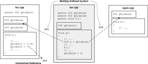
These two situations are shown in Figure 3.9.

foo.cpp
  // definition of the max() function
  int max(int a, int b)
  {
  return (a > b)? a : b;
  }
  // definition of the min() function
  int min(int a, int b)
  {
  return (a <= b)? a : b;
  }

foo.h
 extern int max(int a, int b); // a function declaration
 int min(int a, int b); // also a declaration (the extern //
    is optional/assumed)

foo.cpp
 // All of these are variable definitions:
 U32 gGlobalInteger = 5;
 F32 gGlobalFloatArray[16];
 MyClass gGlobalInstance;

foo.h
  // These are all pure declarations:
  extern U32 gGlobalInteger;
  extern F32 gGlobalFloatArray[16];
  extern MyClass gGlobalInstance;

foo.h
  // This function definition will be inlined properly.
  inline int max(int a, int b)
  {
   return (a > b)? a : b;
  }
  // This declaration cannot be inlined because the
  // compiler cannot “see” the body of the function.
  inline int min(int a, int b);
foo.cpp
  // The body of min() is effectively “hidden” from the
  // compiler, so it can ONLY be inlined within foo.cpp.
  int min(int a, int b)
  {
   return (a <= b)? a : b;
  }

foo.cpp
  // This variable can be used by other .cpp files
  // (external linkage).
  U32 gExternalVariable;
  // This variable is only usable within foo.cpp (internal
  // linkage).
  static U32 gInternalVariable;
  // This function can be called from other .cpp files
  // (external linkage).
  void externalFunction()
  {
    // …
  }
  // This function can only be called from within foo.cpp
  // (internal linkage).
  static void internalFunction()
  {
  // …
  }
bar.cpp
  // This declaration grants access to foo.cpp’s variable.
  extern U32 gExternalVariable;
  // This ‘gInternalVariable’ is distinct from the one
  // defined in foo.cpp -- no error. We could just as
  // well have named it gInternalVariableForBarCpp -- the
  // net effect is the same.
  static U32 gInternalVariable;
  // This function is distinct from foo.cpp’s
  // version -- no error. It acts as if we had named it
  // internalFunctionForBarCpp().
static void internalFunction()
  {
    // …
  }
  // ERROR -- multiply defined symbol!
  void externalFunction()
  {
    // …
  }

3.3.5.1 Executable Image

When a C/C++ program is built, the linker creates an executable file. Most UNIX-like operating systems, including many game consoles, employ a popular executable file format called the executable and linking format (ELF). Executable files on those systems therefore have a .elf extension. The Windows executable format is similar to the ELF format; executables under Windows have a .exe extension. Whatever its format, the executable file always contains a partial image of the program as it will exist in memory when it runs. I say a “partial” image because the program generally allocates memory at runtime in addition to the memory laid out in its executable image.

The executable image is divided into contiguous blocks called segments or sections. Every operating system lays things out a little differently, and the layout may also differ slightly from executable to executable on the same operating system. But the image is usually comprised of at least the following four segments:

Global variables (variables defined at file scope outside any function or class declaration) are stored in either the data or BSS segments, depending on whether or not they have been initialized. The following global will be stored in the data segment, because it has been initialized:

foo.cpp
  F32 gInitializedGlobal = −2.0f;

and the following global will be allocated and initialized to zero by the operating system, based on the specifications given in the BSS segment, because it has not been initialized by the programmer:

foo.cpp
  F32 gUninitializedGlobal;

We’ve seen that the static keyword can be used to give a global variable or function definition internal linkage, meaning that it will be “hidden” from other translation units. The static keyword can also be used to declare a global variable within a function. A function-static variable is lexically scoped to the function in which it is declared (i.e., the variable’s name can only be “seen” inside the function). It is initialized the first time the function is called (rather than before main() is called, as with file-scope statics). But in terms of memory layout in the executable image, a function-static variable acts identically to a file-static global variable—it is stored in either the data or BSS segment based on whether or not it has been initialized.

void readHitchhikersGuide(U32 book)
{
  static U32 sBooksInTheTrilogy =5; // data segment
  static U32 sBooksRead;   // BSS segment
  // …
}

3.3.5.2 Program Stack

When an executable program is loaded into memory and run, the operating system reserves an area of memory for the program stack. Whenever a function is called, a contiguous area of stack memory is pushed onto the stack—we call this block of memory a stack frame. If function a() calls another function b(), a new stack frame for b() is pushed on top of a()’s frame. When b() returns, its stack frame is popped, and execution continues wherever a() left off.

A stack frame stores three kinds of data:

Pushing and popping stack frames is usually implemented by adjusting the value of a single register in the CPU, known as the stack pointer. Figure 3.10 illustrates what happens when the functions shown below are executed.

void c()
{
  U32 localC1;
  // …
}
F32 b()
{
  F32 localB1;
  I32 localB2;
  // …
  c();
  // …
  return localB1;
}

void a()
{
  U32 aLocalsA1[];
  // …
  F32 localA2 = b();
  // …
}

When a function containing automatic variables returns, its stack frame is abandoned and all automatic variables in the function should be treated as if they no longer exist. Technically, the memory occupied by those variables is still there in the abandoned stack frame—but that memory will very likely be overwritten as soon as another function is called. A common error involves returning the address of a local variable, like this:

U32* getMeaningOfLife()
{
  U32 anInteger = 42;
  return &anInteger;
}

You might get away with this if you use the returned pointer immediately and don’t call anyother functions in the interim. But more often than not, this kind of code will crash—sometimes in ways that can be difficult to debug.

3.3.5.3 Dynamic Allocation Heap

Thus far, we’ve seen that a program’s data can be stored as global or static variables or as local variables. The globals and statics are allocated within the executable image, as defined by the data and BSS segments of the executable file. The locals are allocated on the program stack. Both of these kinds of storage are statically defined, meaning that the size and layout of the memory is known when the program is compiled and linked. However, a program’s memory requirements are often not fully known at compile time. A program usually needs to allocate additional memory dynamically.

To allow for dynamic allocation, the operating system maintains a block of memory for each running process from which memory can be allocated by calling malloc() (or an OS-specific function like HeapAlloc() under Windows) and later returned for reuse by the process at some future time by calling free() (or an OS-specific function like HeapFree()). This memory block is known as heap memory, or the free store. When we allocate memory dynamically, we sometimes say that this memory resides on the heap.

In C++, the global new and delete operators are used to allocate and free memory to and from the free store. Be wary, however—individual classes may overload these operators to allocate memory in custom ways, and even the global new and delete operators can be overloaded, so you cannot simply assume that new is always allocating from the global heap.

We will discuss dynamic memory allocation in more depth in Chapter 7. For additional information, see http://en.wikipedia.org/wiki/Dynamic_memory_allocation.

3.3.6.1 Class-Static Members

As we’ve seen, the static keyword has many different meanings depending on context:

Notice that when static is used inside a class declaration, it does not control the visibility of the variable (as it does when used at file scope)—rather, it differentiates between regular per-instance member variables and per-class variables that act like globals. The visibility of a class-static variable is determined by the use of public:, protected: or private: keywords in the class declaration. Class-static variables are automatically included within the namespace of the class or struct in which they are declared. So the name of the class or struct must be used to disambiguate the variable whenever it is used outside that class or struct (e.g., Foo::sVarName).

Like an extern declaration for a regular global variable, the declaration of a class-static variable within a class allocates no memory. The memory for the class-static variable must be defined in a .cpp file. For example:

foo.h
 class Foo
 {
 public:
  static F32 sClassStatic; // allocates no
      // memory!
 };
foo.cpp
 F32 Foo::sClassStatic = -1.0f; // define memory and
     // initialize

3.3.7.1 Alignment and Packing

As we start to think more carefully about the layout of our structs and classes in memory, we may start to wonder what happens when small data members are interspersed with larger members. For example:

struct InefficientPacking
{
  U32 mU1; // 32 bits
  F32 mF2; // 32 bits
  U8 mB3; // 8 bits
  I32 mI4; // 32 bits
  bool mB5; // 8 bits
  char* mP6; // 32 bits
};

You might imagine that the compiler simply packs the data members into memory as tightly as it can. However, this is not usually the case. Instead, the compiler will typically leave “holes” in the layout, as depicted in Figure 3.13. (Some compilers can be requested not to leave these holes by using a preprocessor directive like #pragma pack, or via command-line options; but the default behavior is to space out the members as shown in Figure 3.13.)

Why does the compiler leave these “holes”? The reason lies in the fact that every data type has a natural alignment, which must be respected in order to permit the CPU to read and write memory effectively. The alignment of a data object refers to whether its address in memory is a multiple of its size (which is generally a power of two):

Alignment is important because many modern processors can actually only read and write properly aligned blocks of data. For example, if a program requests that a 32-bit (4-byte) integer be read from address 0x6A341174, the memory controller will load the data happily because the address is 4-byte aligned (in this case, its least significant nibble is 0x4). However, if a request is made to load a 32-bit integer from address 0x6A341173, the memory controller now has to read two 4-byte blocks: the one at 0x6A341170 and the one at 0x6A341174. It must then mask and shift the two parts of the 32-bit integer and logically OR them together into the destination register on the CPU. This is shown in Figure 3.14.

Some microprocessors don’t even go this far. If you request a read or write of unaligned data, you might just get garbage. Or your program might just crash altogether! (The PlayStation 2 is a notable example of this kind of intolerance for unaligned data.)

Different data types have different alignment requirements. A good rule of thumb is that a data type should be aligned to a boundary equal to the width of the data type in bytes. For example, 32-bit values generally have a 4-byte alignment requirement, 16-bit values should be 2-byte aligned, and 8-bit values can be stored at any address (1-byte aligned). On CPUs that support SIMD vector math, the vector registers each contain four 32-bit floats, for a total of 128 bits or 16 bytes. And as you would guess, a four-float SIMD vector typically has a 16-byte alignment requirement.

This brings us back to those “holes” in the layout of structInefficient Packing shown in Figure 3.13. When smaller data types like 8-bit bools are interspersed with larger types like 32-bit integers or floats in a structure or class, the compiler introduces padding (holes) in order to ensure that everything is properly aligned. It’s a good idea to think about alignment and packing when declaring your data structures. By simply rearranging the members of struct InefficientPacking from the example above, we can eliminate some of the wasted padding space, as shown below and in Figure 3.15:

struct MoreEfficientPacking
{
  U32 mU1; // 32 bits (4-byte aligned)
  F32 mF2; // 32 bits (4-byte aligned)
  I32 mI4; // 32 bits (4-byte aligned)
  char* mP6; // 32 bits (4-byte aligned)
  U8 mB3; // 8 bits (1-byte aligned)
  bool mB5; // 8 bits (1-byte aligned)
};

You’ll notice in Figure 3.15 that the size of the structure as a whole is now 20 bytes, not 18 bytes as we might expect, because it has been padded by two bytes at the end. This padding is added by the compiler to ensure proper alignment of the structure in an array context. That is, if an array of these structs is defined and the first element of the array is aligned, then the padding at the end guarantees that all subsequent elements will also be aligned properly.

The alignment of a structure as a whole is equal to the largest alignment requirement among its members. In the example above, the largest member alignment is 4-byte, so the structure as a whole should be 4-byte aligned. I usually like to add explicit padding to the end of my structs to make the wasted space visible and explicit, like this:

struct BestPacking
{
  U32 mU1;  // 32 bits (4-byte aligned)
  F32 mF2;  // 32 bits (4-byte aligned) I32 mI4;  // 32 bits (4-byte aligned)
  char* mP6;  // 32 bits (4-byte aligned)
  U8 mB3;  // 8 bits (1-byte aligned) bool mB5;  // 8 bits (1-byte aligned)
  U8 _pad[2]; // explicit padding
};

3.3.7.2 Memory Layout of C++ Classes

Two things make C++ classes a little different from C structures in terms of memory layout: inheritance and virtual functions.

When class B inherits from class A, B’s data members simply appear immediately after A’s in memory, as shown in Figure 3.16. Each new derived class simply tacks its data members on at the end, although alignment requirements may introduce padding between the classes. (Multiple inheritance does some whacky things, like including multiple copies of a single base class in the memory layout of a derived class. We won’t cover the details here, because game programmers usually prefer to avoid multiple inheritance altogether anyway.)

If a class contains or inherits one or more virtual functions, then four additional bytes (or eight bytes if the target hardware uses 64-bit addresses) are added to the class layout, typically at the very beginning of the class’ layout. These four or eight bytes are collectively called the virtual table pointer or vpointer, because they contain a pointer to a data structure known as the virtual function table or vtable. The vtable for a particular class contains pointers to all the virtual functions that it declares or inherits. Each concrete class has its own virtual table, and every instance of that class has a pointer to it, stored in its vpointer.

The virtual function table is at the heart of polymorphism, because it allows code to be written that is ignorant of the specific concrete classes it is dealing with. Returning to the ubiquitous example of a Shape base class with derived classes for Circle, Rectangle and Triangle, let’s imagine that Shape defines a virtual function called Draw(). The derived classes all override this function, providing distinct implementations named Circle::Draw(), Rectangle::Draw() and Triangle::Draw(). The virtual table for any class derived from Shape will contain an entry for the Draw() function, but that entry will point to different function implementations, depending on the concrete class. Circle’s vtable will contain a pointer to Circle::Draw(), while Rectangle’s virtual table will point to Rectangle::Draw(), and Triangle’s vtable will point to Triangle::Draw(). Given an arbitrary pointer to a Shape (Shape* pShape), the code can simply dereference the vtable pointer, look up the Draw() function’s entry in the vtable, and call it. The result will be to call Circle::Draw() when pShape points to an instance of Circle, Rectangle::Draw() when pShape points to a Rectangle, and Triangle::Draw() when pShape points to a Triangle.

These ideas are illustrated by the following code excerpt. Notice that the base class Shape defines two virtual functions, SetId() and Draw(), the latter of which is declared to be pure virtual. (This means that Shape provides no default implementation of the Draw() function, and derived classes must override it if they want to be instantiable.) Class Circle derives from Shape, adds some data members and functions to manage its center and radius, and overrides the Draw() function; this is depicted in Figure 3.17. Class Triangle also derives from Shape. It adds an array of Vector3 objects to store its three vertices and adds some functions to get and set the individual vertices. Class Triangle overrides Draw() as we’d expect, and for illustrative purposes it also overrides SetId(). The memory image generated by the Triangle class is shown in Figure 3.18.

class Shape
{
public:
 virtual void SetId(int id) {m_id = id;}
 int   GetId() const {return m_id;}
 virtual void Draw() = 0; // pure virtual -- no impl.
private:
 int m_id;
};
class Circle : public Shape
{
public:
 void  SetCenter(const Vector3& c) {m_center=c;}
 Vector3 GetCenter() const {return m_center;}
 void  SetRadius(float r) {m_radius = r;}
 float  GetRadius() const {return m_radius;}
 virtual void Draw()
 {
   // code to draw a circle
 }
private:
 Vector3 m_center;
 float m_radius;
};
class Triangle : public Shape
{
public:
 void SetVertex(int i, const Vector3& v);
 Vector3 GetVertex(int i) const {return m_vtx[i];}
 virtual void Draw()
{
   // code to draw a triangle
}
virtual void SetId(int id)
{
  // call base class’ implementation
  Shape::SetId(id);
  // do additional work specific to Triangles…
}
private:
  Vector3 m_vtx[3];
};
// -------------------------
void main(int, char**)
{
 Shape* pShape1 = new Circle;
 Shape* pShape2 = new Triangle;
 pShape1->Draw();
 pShape2->Draw();
 // …
}

3.4.3.1 ALU

The ALU performs unary and binary arithmetic operations such as negation, addition, subtraction, multiplication and division, and also performs logical operations such as AND, OR, exclusive OR (abbreviated XOR or EOR), bitwise complement and bit shifting. In some CPU designs, the ALU is physically split into an arithmetic unit (AU) and a logic unit (LU).

An ALU typically performs integer operations only. Floating-point calculations require very different circuitry, and are usually performed by a physically separate floating-point unit (FPU). Early CPUs like the Intel 8088/8086 had no on-chip FPU; if floating-point math support was desired, these CPUs had to be augmented with a separate FPU co-processor chip such as the Intel 8087. In later CPU designs, an FPU was typically included on the main CPU die.

3.4.3.2 VPU

A vector processing unit (VPU) acts a bit like a combination ALU/FPU, in that it can typically perform both integer and floating-point arithmetic. What differentiates a VPU is its ability to apply arithmetic operators to vectors of input data—each of which typically consists of between two and 16 floatingpoint values or up to 64 integer values of various widths—rather than to scalar inputs. Vector processing is also known as single instruction multiple data or SIMD, because a single arithmetic operator (e.g, multiplication) is applied to multiple pairs of inputs simultaneously. See Section 4.10 for more details.

Today’s CPUs don’t actually contain an FPU per se. Instead, all floatingpoint calculations, even those involving scalar float values, are performed by the VPU. Eliminating the FPU reduces the transistor count on the CPU die, allowing those transistors to be used to implement larger caches, more-complex out-of-order execution logic, and so on. And as we’ll see in Section 4.10.6, optimizing compilers will typically convert math performed on float variables into vectorized code that uses the VPU anyway.

3.4.3.3 Registers

In order to maximize performance, an ALU or FPU can usually only perform calculations on data that exists in special high-speed memory cells called registers. Registers are typically physically separate from the computer’s main memory, located on-chip and in close proximity to the components that access them. They’re usually implemented using fast, high-cost multi-ported static RAM or SRAM. (See Section 3.4.5 for more information about memory technologies.) A bank of registers within a CPU is called a register file.

Because registers aren’t part of main memory,¹ they typically don’t have addresses but they do have names. These could be as simple as R0, R1, R2 etc., although early CPUs tended to use letters or short mnemonics as register names. For example, the Intel 8088/8086 had four 16-bit general-purpose registers named AX, BX, CX and DX. The 6502 by MOS Technology, Inc. performed all of its arithmetic operations using a register known as the accumulator² (A), and used two auxillary registers called X and Y for other operations such as indexing into an array.

Some of the registers in a CPU are designed to be used for general calculations. They’re appropriately named general-purpose registers (GPR). Every CPU also contains a number of special-purpose registers (SPR). These include:

3.4.3.4 Control Unit

If the CPU is the “brains” of the computer, then the control unit (CU) is the “brains” of the CPU. Its job is to manage the flow of data within the CPU, and to orchestrate the operation of all of the CPU’s other components.

The CU runs a program by reading a stream of machine language instructions, decoding each instruction by breaking it into its opcode and operands, and then issuing work requests and/or routing data to the ALU, FPU, VPU, the registers and/or the memory controller as dictated by the current instruction’s opcode. In pipelined and superscalar CPUs, the CU also conains complex circuitry to handle branch prediction and the scheduling of instructions for out-of-order execution. We’ll look at the operation of the CU in more detail in Section 3.4.7.

3.4.4.1 Clock Speed versus Processing Power

The “processing power” of a CPU or computer can be defined in various ways. One common measure is the throughput of the machine—the number of operations it can perform during a given interval of time. Throughput is expressed either in units of millions of instructions per second (MIPS) or floating-point operations per second (FLOPS).

Because instructions or floating-point operations don’t generally complete in exactly one cycle, and because different instructions take differing numbers of cycles to run, the MIPS or FLOPS metrics of a CPU are just averages. As such, you cannot simply look at the clock frequency of a CPU and determine its processing power in MIPS or FLOPS. For example, a serial CPU running at 3 GHz, in which one floating-point multiply takes six cycles to complete on average, could theoretically achieve 0.5 GFLOPS. But many factors including pipelining, superscalar designs, vector processing, multicore CPUs and other forms of parallelism conspire to obfuscate the relationship between clock speed and processing power. Thus the only way to determine the true processing power of a CPU or computer is to measure it—typically by running standardized benchmarks.

3.4.5 Memory

The memory in a computer acts like a bank of mailboxes at the post office, with each box or “cell” typically containing a single byte of data (an eight-bit value).⁴ Each one-byte memory cell is identified by its address—a simple numbering scheme ranging from 0 to N − 1, where N is the size of addressable memory in bytes.

Memory comes in two basic flavors:

ROM modules retain their data even when power is not applied to them. Some types of ROM can be programmed only once. Others, known as electronically erasable programmable ROM or EEPROM, can be reprogrammed over and over again. (Flash drives are one example of EEPROM memory.)

RAM can be further divided into static RAM (SRAM) and dynamic RAM (DRAM). Both static and dynamic RAM retain their data as long as power is applied to them. But unlike static RAM, dynamic RAM also needs to be “refreshed” periodically (by reading the data and then re-writing it) in order to prevent its contents from disappearing. This is because DRAM memory cells are built from MOS capacitors that gradually lose their charge, and reading such memory cells is destructive to the data they contain.

RAM can also be categorized by various other design characteristics, such as:

3.4.6.1 Bus Widths

The width of the address bus, measured in bits, controls the range of possible addresses that can be accessed by the CPU (i.e., the size of addressable memory in the machine). For example, a computer with a 16-bit address bus can access at most 64 KiB of memory, using addresses in the range 0x0000 through 0xFFFF. A computer with a 32-bit address bus can access a 4 GiB memory, using addresses in the range 0x00000000 through 0xFFFFFFFF. And a machine with a 64-bit address bus can access a staggering 16 EiB (exbibytes) of memory. That’s 2⁶⁴ = 16 × 1024⁶ ≈ 1.8 × 10¹⁹ bytes!

The width of the data bus determines how much data can be transferred between CPU registers and memory at a time. (The data bus is typically the same width as the general-purpose registers in the CPU, although this isn’t always the case.) An 8-bit data bus means that data can be transferred one byte at a time—loading a 16-bit value from memory would require two separate memory cycles, one to fetch the least-significant byte and one to fetch the most-significant byte. At the other end of the spectrum, a 64-bit data bus can transfer data between memory and a 64-bit register as a single memory operation.

It’s possible to access data items that are narrower than the width of a machine’s data bus, but it’s typically more costly than accessing items whose widths match that of the data bus. For example, when reading a 16-bit value on a 64-bit machine, a full 64 bits worth of data must still be read from memory. The desired 16-bit field then has to be masked off and possibly shifted into place within the destination register. This is one reason why the C language does not define an int to be a specific number of bits wide—it was purposefully defined to match the “natural” size of a word on the target machine, in an attempt to make source code more portable. (Ironically this policy has actually resulted in source code often being less portable due to implicit assumptions about the width of an int.)

3.4.6.2 Words

The term “word” is often used to describe a multi-byte value. However, the number of bytes comprising a word is not universally defined. It depends to some degree on context.

Sometimes the term “word” refers to the smallest multi-byte value, namely 16 bits or two bytes. In that context, a double word would be 32 bits (four bytes) and a quad word would be 64 bits (eight bytes). This is the way the term “word” is used in the Windows API.

On the other hand, the term “word” is also used to refer to the “natural” size of data items on a particular machine. For example, a machine with 32-bit registers and a 32-bit data bus operates most naturally with 32-bit (four byte) values, and programmers and hardware folks will sometimes say that such a machine as a word size of 32 bits. The takeaway here is to be aware of context whenever you hear the term “word” being used to refer to the size of a data item.

3.4.6.3 n-Bit Computers

You may have encountered the term “n-bit computer.” This usually means a machine with an n-bit data bus and/or registers. But the term is a bit ambiguous, because it might also refer to a computer whose address bus is n bits wide. Also, on some CPUs the data bus and register widths don’t match. For example, the 8088 had 16-bit registers and a 16-bit address bus, but it only had an 8-bit data bus. Hence it acted like a 16-bit machine internally, but its 8-bit data bus caused it to behave like an 8-bit machine in terms of memory accesses. Again, be aware of context when talking about an n-bit machine.

3.4.7.1 Instruction Set Architecture (ISA)

CPU designs vary widely from one manufacturer to the next. The set of all instructions supported by a given CPU, along with various other details of the CPU’s design like its addressing modes and the in-memory instruction format, is called its instruction set architecture or ISA. (This is not to be confused with a programming language’s application binary interface or ABI, which defines higher-level protocols like calling conventions.) We won’t attempt to cover the details of any one CPU’s ISA here, but the following categories of instruction types are common to pretty much every ISA:

We can’t possibly list all instruction types here, but if you’re curious you can always read through the ISA documentation of a real processor like the Intel x86 (which is available at http://intel.ly/2woVFQ8).

3.4.7.2 Machine Language

Computers can only deal with numbers. As such, each instruction in a program’s instruction stream must be encoded numerically. When a program is encoded in this way, we say it is written in machine language, or ML for short. Of course, machine language isn’t a single language—it’s really a multitude of languages, one for each distinct CPU/ISA.

Every machine language instruction is comprised of three basic parts:

Operands come in many flavors. Some instructions might take the names (encoded as numeric ids) of one or more registers as operands. Others might expect a literal value as an operand (e.g., “load the value 5 into register R2,” or “jump to address 0x0102ED5C”). The way in which an instruction’s operands are interpreted and used by the CPU is known as the instruction’s addressing mode. We’ll discuss addressing modes in more detail in Section 3.4.7.4.

The opcode and operands (if any) of an ML instruction are packed into a contiguous sequence of bits called an instruction word. A hypothetical CPU might encode its instructions as shown in Figure 3.21 with perhaps the first byte containing the opcode, addressing mode and various options flags, followed by some number of bytes for the operands. Each ISA defines the width of an instruction word (i.e., the number of bits occupied by each instruction) differently. In some ISAs, all instructions occupy a fixed number of bits; this is typical of reduced instruction set computers (RISC). In other ISAs, different types of instructions may be encoded into differently-sized instruction words; this is common in complex instruction set computers (CISC).

Instruction words can be as small as four bits in some microcontrollers, or they may be many bytes in size. Instruction words are often multiples of 32 or 64 bits, because this matches the width of the CPU’s registers and/or data bus. In very long instruction word (VLIW) CPU designs, parallelism is achieved by allowing multiple operations to be encoded into a single very wide instruction word, for the purpose of executing them in parallel. Instructions in a VLIW ISA can therefore be upwards of hundreds of bytes in width.

For a concrete example of machine language instruction encoding on the Intel x86 ISA, see http://aturing.umcs.maine.edu/∼meadow/courses/cos335/Asm07-MachineLanguage.pdf.

3.4.7.3 Assembly Language

Writing a program directly in machine language is tedious and error-prone. To make life easier for programmers, a simple text-based version of machine language was developed called assembly language. In assembly language, each instruction within a given CPU’s ISA is given a mnemonic—a short English word or abbreviation that is much easier to remember than corresponding numeric opcode. Instruction operands can be specified conveniently as well: Registers can be referred to by name (e.g., R0 or EAX), and memory addresses can be written in hex, or assigned symbolic names much like the global variables of higher-level languages. Locations in the assembly program can be tagged with human-readable labels, and jump/branch instructions refer to these labels rather than to raw memory addresses.

An assembly language program consists of a sequence of instructions, each comprised of a mnemonic and zero or more operands, listed in a text file with one instruction per line. A tool known as an assembler reads the program source file and converts it into the numeric ML representation understood by the CPU. For example, an assembly language program that implements the following snippet of C code:

if (a > b)
  return a + b;
else
  return 0;

could be implemented by an assembly language program that looks something like this:

; if (a > b)
cmp eax, ebx ; compare the values
jle ReturnZero ; jump if less than or equal
; return a + b;
add eax, ebx ; add & store result in EAX
ret   ; (EAX is the return value)
ReturnZero:
  ; else return 0;
xor eax, eax; set EAX to zero
ret   ; (EAX is the return value)

Let’s breakthis down. The cmp instruction compares the values inregisters EAX and EBX (which we’re assuming contain the values a and b from the C snippet). Next, the jle instruction branches to the label ReturnZero, but it does so if and only if the value in EAX is less than or equal to EBX. Otherwise it falls through.

If EAX is greater than EBX (a > b), we fall through to the add instruction, which calculates a + b and stores the result back into EAX, which we’re assuming serves as the return value. We issue a ret instruction, and control is returned to the calling function.

If EAX is less than or equal to EBX (a <= b), the branch is taken and we continue execution immediately after the label ReturnZero. Here, we use a little trick to set EAX to zero by XORing it with itself. Then we issue a ret instruction to return that zero to the caller.

For more details on Intel assembly language programming, see http://www.cs.virginia.edu/∼evans/cs216/guides/x86.html.

3.4.7.4 Addressing Modes

A seemingly simple instruction like “move” (which transfers data between registers and memory) has many different variants. Are we moving a value from one register to another? Are we loading a literal value like 5 into a register? Are we loading a value from memory into a register? Or are we storing a value in a register out to memory? All of these variants are called addressing modes. We won’t go over all the possible addressing modes here, but the following list should give you a good feel for the kinds of addressing modes you will encounter on a real CPU:

3.4.7.5 Further Reading on Assembly Language

In the preceding sections, we’ve had just a tiny taste of assembly language. For an easy-to-digest description of x86 assembly programming, see http://flint.cs.yale.edu/cs421/papers/x86-asm/asm.html. For more on calling conventions and ABIs, see https://en.wikibooks.org/wiki/X86_Disassembly/Functions_and_Stack_Frames.

3.5.1.1 Memory-Mapped I/O

Address ranges needn’t all map to memory devices—an address range might also be mapped to other peripheral devices, such as a joypad or a network interace card (NIC). This approach is called memory-mapped I/O because the CPU can perform I/O operations on a peripheral device by reading or writing to addresses, just as if they were oridinary RAM. Under the hood, special circuitry detects that the CPU is reading from or writing to a range of addresses that have been mapped to a non-memory device, and converts the read or write request into an I/O operation directed at the device in question. As a concrete example, the Apple II mapped I/O devices into the address range 0xC000 through 0xC0FF, allowing programs to do things like control bank-switched RAM, read and control voltages on the pins of a game controller socket on the motherboard, and perform other I/O operations by merely reading from and writing to the addresses in this range.

Alternatively, a CPU might communicate with non-memory devices via special registers known as ports. In this case, whenever the CPU requests that data be read from or written to a port register, the hardware converts the request into an I/O operation on the target device. This approach is called port-mapped I/O. In the Arduino line of microcontrollers, port-mapped I/O gives a program direct control over the digital inputs and outputs at some of the pins of the chip.

3.5.1.2 Video RAM

Raster-based display devices typically read a hard-wired range of physical memory addresses in order to determine the brightness/color of each pixel on the screen. Likewise, early charcter-based displays would determine which character glyph to display at each location on the screen by reading ASCII codes from a block of memory. A range of memory addresses assigned for use by a video controller is known as video RAM (VRAM).

In early computers like the Apple II and early IBM PCs, video RAM used to correspond to memory chips on the motherboard, and memory addresses in VRAM could be read from and written to by the CPU in exactly the same way as any other memory location. This is also the case on game consoles like the PlayStation 4 and the Xbox One, where both the CPU and GPU share access to a single, large block of unified memory.

In personal computers, the GPU often lives on a separate circuit board, plugged into an expansion slot on the motherboard. Video RAM is typically located on the video card so that the GPU can access it as quickly as possible. A bus protocol such as PCI, AGP or PCI Express (PCIe) is used to transfer data back and forth between “main RAM” and VRAM, via the expansion slot’s bus. This physical separation between main RAM and VRAM can be a significant performance bottleneck, and is one of the primary contributors to the complexity of rendering engines and graphics APIs like OpenGL and DirectX 11.

3.5.1.3 Case Study: The Apple II Memory Map

To illustrate the concepts of memory mapping, let’s look at a simple real-world example. The Apple II had a 16-bit address bus, meaning that its address space was only 64 KiB in size. This address space was mapped to ROM, RAM, memory-mapped I/O devices and video RAM regions as follows:

0xC100 - 0xFFFF ROM (Firmware)
0xC000 - 0xC0FF Memory-Mapped I/O
0x6000 - 0xBFFF General-purpose RAM
0x4000 - 0x5FFF High-res video RAM (page 2)
0x2000 - 0x3FFF High-res video RAM (page 1)
0x0C00 - 0x1FFF General-purpose RAM
0x0800 - 0x0BFF Text/lo-res video RAM (page 2)
0x0400 - 0x07FF Text/lo-res video RAM (page 1)
0x0200 - 0x03FF General-purpose and reserved RAM
0x0100 - 0x01FF Program stack
0x0000 - 0x00FF Zero page (mostly reserved for DOS)

We should note that the addresses in the Apple II memory map corresponded directly to memory chips on the motherboard. In today’s operating systems, programs work in terms of virtual addresses rather than physical addresses. We’ll explore virtual memory in the next section.

3.5.2.1 Virtual Memory Pages

To understand how this remapping takes place, we need to imagine that the entire addressable memory space (that’s 2ⁿ byte-sized cells if the address bus is n bits wide) is conceptually divided into equally-sized contiguous chunks known as pages. Page sizes differ from OS to OS, but are always a power of two—a typical page size is 4 KiB or 8 KiB. Assuming a 4 KiB page size, a 32-bit address space would be divided up into 1,048,576 distinct pages, numbered from 0x0 to 0xFFFFF, as shown in Table 3.2.

The mapping between virtual addresses and physical addresses is always done at the granularity of pages. One hypothetical mapping between virtual and physical addresses is illustrated in Figure 3.22.

3.5.2.2 Virtual to Physical Address Translation

Whenever the CPU detects a memory read or write operation, the address is split into two parts: the page index and an offset within that page (measured in bytes). For a page size of 4 KiB, the offset is just the lower 12 bits of the address, and the page index is the upper 20 bits, masked off and shifted to the right by 12 bits. For example, the virtual address 0x1A7C6310 corresponds to an offset of 0x310 and a page index of 0x1A7C6.

The page index is then looked up by the CPU’s memory management unit (MMU) in a page table that maps virtual page indices to physical ones. (The page table is stored in RAM and is managed by the operating system.) If the page in question happens to be mapped to a physical memory page, the virtual page index is translated into the corresponding physical page index, the bits of this physical page index are shifted to the left as appropriate and ORed together with the bits of the original page offset, and voila! We have a physical address. So to continue our example, if virtual page 0x1A7C6 happens to map to physical page 0x73BB9, then the translated physical address would end up being 0x73BB9310. This is the address that would actually be transmitted over the address bus. Figure 3.23 illustrates the operation of the MMU.

If the page table indicates that a page is not mapped to physical RAM (either because it was never allocated, or because that page has since been swapped out to a disk file), the MMU raises an interrupt, which tells the operating system that the memory request can’t be fulfilled. This is called a page fault. (See Section 4.4.2 for more on interrupts.)

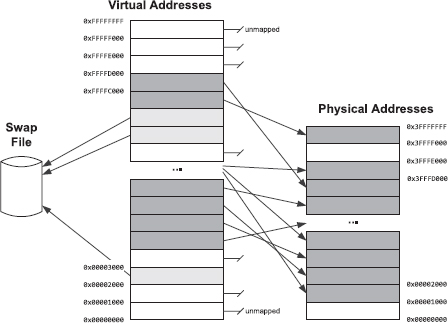
3.5.2.3 Handling Page Faults

For accesses to unallocated pages, the OS normally responds to a page fault by crashing the program and generating a core dump. For accesses to pages that have been swapped out to disk, the OS temporarily suspends the currently-running program, reads the page from the swap file into a physical page of RAM, and then translates the virtual address to a physical address as usual. Finally it returns control back to the suspended program. From the point of view of the program, this operation is entirely seamless—it never “knows” whether a page was already in memory or had to be swapped in from disk.

Normally pages are swapped out to disk only when the load on the memory system is high, and physical pages are in short supply. The OS tries to swap out only the least-frequently-used pages of memory to avoid programs continually “thrashing” between memory-based and disk-based pages.

3.5.2.4 The Translation Lookaside Buffer (TLB)

Because page sizes tend to be small relative to the total size of addressable memory (typically 4 KiB or 8 KiB), the page table can become very large. Looking up physical addresses in the page table would be time-consuming if the entire table had to be scanned for every memory access a program makes.

To speed up access, a caching mechanism is used, based on the assumption that an average program will tend to reuse addresses within a relatively small number of pages, rather than read and write randomly across the entire address range. A small table known as the translation lookaside buffer (TLB) is maintained within the MMU on the CPU die, in which the virtual-to-physical address mappings of the most recently-used addresses are cached. Because this buffer is located in close proximity to the MMU, accessing it is very fast.

The TLB acts a lot like a general-purpose memory cache hierarchy, except that it is only used for caching page table entries. See Section 3.5.4 for a discussion of how cache hierarchies work.

3.5.2.5 Further Reading on Virtual Memory

See https://www.cs.umd.edu/class/sum2003/cmsc311/Notes/Memory/virtual.html and https://gabrieletolomei.wordpress.com/miscellanea/operating-systems/virtual-memory-paging-and-swapping for two good discussions of virtual memory implementation details.

This paper by Ulrich Drepper entitled, “What Every Programmer Should Know About Memory” is also a must-read for all programmers: https://www.akkadia.org/drepper/cpumemory.pdf.

3.5.3.1 The Memory Gap

In the early days of computing, memory access latency and instruction execution latency were on roughly equal footing. For example, on the Intel 8086, register-based instructions could execute in two to four cycles, and a main memory access also took roughly four cycles. However, over the past few decades both raw clock speeds and the effective instruction throughput of CPUs have been improving at a much faster rate than memory access speeds. Today, the access latency of main memory is extremely high relative to the latency of executing a single instruction: Whereas a register-based instruction still takes between one and 10 cycles to complete on an Intel Core i7, an access to main RAM can take on the order of 500 cycles to complete! This ever-increasing discrepancy between CPU speeds and memory access latencies is often called the memory gap. Figure 3.24 illustrates the trend of an ever-increasing memory gap over time.

Programmers and hardware designers have together developed a wide range of techniques to work around the problems caused by high memory access latency. These techniques usually focus on one or more of the following:

In this section, we’ll have a closer look at memory architectures for average latency reduction. We’ll discuss the other two techniques (latency “hiding” and the minimization of memory accesses via judicious data layout) while investigating parallel hardware design and concurrent programming techniques in Chapter 4.

3.5.3.2 Register Files

A CPU’s register file is perhaps the most extreme example of a memory architecture designed to minimize access latency. Registers are typically implemented using multi-ported static RAM (SRAM), usually with dedicated ports for read and write operations, allowing these operations to occur in parallel rather than serially. What’s more, the register file is typically located immediately adjacent to the circuitry for the ALU that uses it. Furthermore, registers are accessed pretty much directly by the ALU, whereas accesses to main RAM typically have to pass through the virtual address translation system, the memory cache hierarchy and cache coherence protocol (see Section 3.5.4), the address and data buses, and possibly also through crossbar switching logic. These facts explain why registers can be accessed so quickly, and also why the cost of register RAM is relatively high as compared to general-purpose RAM. This higher cost is justified because registers are by far the most frequently-used memory in any computer, and because the total size of the register file is very small when compared to the size of main RAM.

3.5.4.1 Cache Lines

Memory caching takes advantage of the fact that memory access patterns in real software tend to exhibit two kinds of locality of reference:

To take advantage of locality of reference, memory caching systems move data into the cache in contiguous blocks called cache lines rather than caching data items individually.

For example, let’s say the program is accessing the data members of an instance of a class or struct. When the first member is read, it might take hundreds of cycles for the memory controller to reach out into main RAM to retrieve the data. However, the cache controller doesn’t just read that one member—it actually reads a larger contiguous block of RAM into the cache. That way, subsequent reads of the other data members of the instance will likely result in low-cost cache hits.

3.5.4.2 Mapping Cache Lines to Main RAM Addresses

There is a simple one-to-many correspondence between memory addresses in the cache and memory addresses in main RAM. We can think of the address space of the cache as being “mapped” onto the main RAM address space in a repeating pattern, starting at address 0 in main RAM and continuing on up until all main RAM addresses have been “covered” by the cache.

As a concrete example, let’s say that our cache is 32 KiB in size, and that cache lines are 128 bytes each. The cache can therefore hold 256 cache lines (256 × 128 = 32,768 B = 32 KiB). Let’s further assume that main RAM is 256 MiB in size. So main RAM is 8192 times as big as the cache, because (256 × 1024)/32 = 8192. That means we need to overlay the address space of the cache onto the main RAM address space 8192 times in order to cover all possible physical memory locations. Or put another way, a single line in the cache maps to 8192 distinct line-sized chunks of main RAM.

Given any address in main RAM, we can find its address in the cache by taking the main RAM address modulo the size of the cache. So for a 32 KiB cache and 256 MiB of main RAM, the cache addresses 0x0000 through 0x7FFF (that’s 32 KiB) map to main RAM addresses 0x0000 through 0x7FFF. But this range of cache addresses also maps to main RAM addresses 0x8000 through 0xFFFF, 0x10000 through 0x17FFF, 0x18000 through 0x1FFFF and so on, all the way up to the last main RAM block at addresses 0xFFF8000 through 0xFFFFFFF. Figure 3.25 illustrates the mapping between main RAM and cache RAM.

3.5.4.3 Addressing the Cache

Let’s consider what happens when the CPU reads a single byte from memory. The address of the desired byte in main RAM is first converted into an address within the cache. The cache controller then checks whether or not the cache line containing that byte already exists in the cache. If it does, it’s a cache hit, and the byte is read from the cache rather than from main RAM. If it doesn’t, it’s a cache miss, and the line-sized chunk of data is read from main RAM and loaded into the cache so that subsequent reads of nearby addresses will be fast.

The cache can only deal with memory addresses that are aligned to a multiple of the cache line size (see Section 3.3.7.1 for a discussion of memory alignment). Put another way, the cache can really only be addressed in units of lines, not bytes. Hence we need to convert our byte’s address into a cache line index.

Consider a cache that is 2^M bytes in total size, containing lines that are 2ⁿ in size. The n least-significant bits of the main RAM address represent the offset of the byte within the cache line. We strip off these n least-significant bits to convert from units of bytes to units of lines (i.e., we divide the address by the cache line size, which is 2ⁿ). Finally we split the resulting address into two pieces: The (M − n) least-significant bits become the cache line index, and all the remaining bits tell us from which cache-sized block in main RAM the cache line came from. The block index is known as the tag.

In the case of a cache miss, the cache controller loads a line-sized chunk of data from main RAM into the corresponding line within the cache. The cache also maintains a small table of tags, one for each cache line. This allows the caching system to keep track of from which main RAM block each line in the cache came. This is necessary because of the many-to-one relationship between memory addresses in the cache and memory addresses in main RAM. Figure 3.26 illustrates how the cache associates a tag with each active line within it.

Returning to our example of reading a byte from main RAM, the complete sequence of events is as follows: The CPU issues a read operation. The main RAM address is converted into an offset, line index and tag. The corresponding tag in the cache is checked, using the line index to find it. If the tag in the cache matches the requested tag, it’s a cache hit. In this case, the line index is used to retrieve the line-sized chunk of data from the cache, and the offset is used to locate the desired byte within the line. If the tags do not match, it’s a cache miss. In this case, the appropriate line-sized chunk of main RAM is read into the cache, and the corresponding tag is stored in the cache’s tag table. Subsequent reads of nearby addresses (those that reside within the same cache line) will therefore result in much faster cache hits.

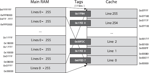
3.5.4.4 Set Associativity and Replacement Policy

The simple mapping between cache lines and main RAM addresses described above is known as a direct-mapped cache. It means that each address in main RAM maps to only one line in the cache. Using our 32 KiB cache with 128-byte lines as an example, the main RAM address 0x203 maps to cache line 4 (because 0x203 is 515, and [515/128] = 4). However, in our example there are 8192 unique cache-line-sized blocks of main RAM that all map to cache line 4. Specifically, cache line 4 corresponds to main RAM addresses 0x200 through 0x27F, but also to addresses 0x8200 through 0x827F, and 0x10200 through 0x1027f, and 8189 other cache-line-sized address ranges as well.

When a cache miss occurs, the CPU must load the corresponding cache line from main memory into the cache. If the line in the cache contains no valid data, we simply copy the data into it and we’re done. But if the line already contains data (from a different main memory block), we must overwrite it. This is known as evicting the cache line.

The problem with a direct-mapped cache is that it can result in pathological cases. For example, two unrelated main memory blocks might keep evicting one another in a ping-pong fashion. We can obtain better average performance if each main memory address can map to two or more distinct lines in the cache. In a 2-way set associative cache, each main RAM address maps to two cache lines. This is illustrated in Figure 3.27. Obviously a 4-way set associative cache performs even better than a 2-way, and an 8-way or 16-way cache can outperform a 4-way cache and so on.

Once we have more than one “cache way,” the cache controller is faced with a dilemma: When a cache miss occurs, which of the “ways” should we evict and which ones should we allow to stay resident in the cache? The answer to this question differs between CPU designs, and is known as the CPU’s replacement policy. One popular policy is not most-recently used (NMRU). In this scheme, the most-recently used “way” is kept track of, and eviction always affects the “way” or “ways” that are not the most-recently used one. Other policies include first in first out (FIFO), which is the only option in a direct-mapped cache, least-recently used (LRU), least-frequently used (LFU), and pseudorandom. For more on cache replacement policies, see https://ece752.ece.wisc.edu/lect11-cache-replacement.pdf.

3.5.4.5 Multilevel Caches

The hit rate is a measure of how often a program hits the cache, as opposed to incurring the large cost of a cache miss. The higher the hit rate, the better the program will perform (all other things being equal). There is a fundamental trade-off between cache latency and hit rate. The larger the cache, the higher the hit rate—but larger caches cannot be located as close to the CPU, so they tend to be slower than smaller ones.

Most game consoles employ at least two levels of cache. The CPU first tries to find the data it’s looking for in the level 1 (L1) cache. This cache is small but has a very low access latency. If the data isn’t there, it tries the larger but higher-latency level 2 (L2) cache. Only if the data cannot be found in the L2 cache do we incur the full cost of a main memory access. Because the latency of main RAM can be so high relative to the CPU’s clock rate, some PCs even include level 3 (L3) and level 4 (L4) caches.

3.5.4.6 Instruction Cache and Data Cache

When writing high-performance code for a game engine or for any other performance-critical system, it is important to realize that both data and code are cached. The instruction cache (I-cache, often denoted I$) is used to preload executable machine code before it runs, while the data cache (D-cache, or D$) is used to speed up read and write operations performed by that machine code. In a level 1 (L1) cache, the two caches are always physically distinct, because it is undesirable for an instruction read to cause valid data to be bumped out of the cache or vice versa. So when optimizing our code, we must consider both D-cache and I-cache performance (although as we’ll see, optimizing one tends to have a positive effect on the other). Higher-level caches (L2, L3, L4) typically do not make this distinction between code and data, because their larger size tends to mitigate the problems of code evicting data or data evicting code.

3.5.4.7 Write Policy

We haven’t talked yet about what happens when the CPU writes data to RAM. How the cache controller handles writes is known as its write policy. The simplest kind of cache is called a write-through cache; in this relatively simple cache design, all writes to the cache are mirrored to main RAM immediately. In a write-back (or copy-back) cache design, data is first written into the cache and the cache line is only flushed out to main RAM under certain circumstances, such as when a dirty cache line needs to be evicted in order to read in a new cache line from main RAM, or when the program explicitly requests a flush to occur.

3.5.4.8 Cache Coherency: MESI, MOESI and MESIF

When multiple CPU cores share a single main memory store, things get more complicated. It’s typical for each core to have its own L1 cache, but multiple cores might share an L2 cache, as well as sharing main RAM. See Figure 3.28 for an illustration of a two-level cache architecture with two CPU cores sharing one main memory store and an L2 cache.

In the presence of multiple cores, it’s important for the system to maintain cache coherency. This amounts to making sure that the data in the caches belonging to multiple cores match one another and the contents of main RAM. Coherency doesn’t have to be maintained at every moment—all that matters is that the running program can never tell that the contents of the caches are out of sync.

The three most common cache coherency protocols are known as MESI (modified, exclusive, shared, invalid), MOESI (modified, owned, exclusive, shared, invalid) and MESIF (modified, exclusive, shared, invalid and forward). We’ll discuss the MESI protocol in more depth when we talk about multicore computing architectures in Section 4.9.4.2.

3.5.4.9 Avoiding Cache Misses

Obviously cache misses cannot be totally avoided, since data has to move to and from main RAM eventually. The trick to writing high performance software in the presence of a memory cache hierarchy is to arrange your data in RAM, and design your data manipulation algorithms, in such a way that the minimum number of cache misses occur.

The best way to avoid D-cache misses is to organize your data in contiguous blocks that are as small as possible and then access them sequentially. When the data is contiguous (i.e., you don’t “jump around” in memory a lot), a single cache miss will load the maximum amount of relevant data in one go. When the data is small, it is more likely to fit into a single cache line (or at least a minimum number of cache lines). And when you access your data sequentially, you avoid evicting and reloading cache lines multiple times.

Avoiding I-cache misses follows the same basic principle as avoiding D-cache misses. However, the implementation requires a different approach. The easiest thing to do is to keep your high-performance loops as small as possible in terms of code size, and avoid calling functions within your innermost loops. If you do opt to call functions, try to keep their code size small too. This helps to ensure that the entire body of the loop, including all called functions, will remain in the I-cache the entire time the loop is running.

Use inline functions judiciously. Inlining a small function can be a big performance boost. However, too much inlining bloats the size of the code, which can cause a performance-critical section of code to no longer fit within the cache.

3.5.5.1 SPU Local Stores on the PS3

The PlayStation 3 is a classic example of a NUMA architecture. The PS3 contains a single main CPU known as the Power processing unit (PPU), eight⁸ coprocessors known as synergistic processing units (SPUs), and an NVIDIA RSX graphics processing unit (GPU). The PPU has exclusive access to 256 MiB of main system RAM (with an L1 and L2 cache), the GPU has exclusive access to 256 MiB of video RAM (VRAM), and each SPU has its own private 256 KiB local store.

The physical address spaces of main RAM, video RAM and the SPUs’ local stores are all totally isolated from one another. This means that, for example, the PPU cannot directly address memory in VRAM or in any of the SPUs’ local stores, and any given SPU cannot directly address main RAM, video RAM, or any of the other SPUs’ local stores, only its own local store. The memory architecture of the PS3 is illustrated in Figure 3.29.

3.5.5.2 PS2 Scratchpad (SPR)

Looking even farther back to the PlayStation 2, we can learn about another memory architecture that was designed to improve overall system performance. The main CPU on the PS2, called the emotion engine (EE), has a special 16 KiB area of memory called the scratchpad (abbreviated SPR), in addition to a 16 KiB L1 instruction cache (I-cache) and an 8 KiB L1 data cache (D-cache). The PS2 also contains two vector coprocessors known as VU0 and VU1, each with their own L11- and D-caches, and a GPU known as the graphics synthesizer (GS) connected to a 4 MiB bank of video RAM. The PS2’s memory architecture is illustrated in Figure 3.30.

The scratchpad is located on the CPU die, and therefore enjoys the same low latency as L1 cache memory. But unlike the L1 cache, the scratchpad is memory-mapped so that it appears to the programmer to be a range of regular main RAM addresses. The scratchpad on the PS2 is itself uncached, meaning that reads and writes from and to it are direct; they bypass the EE’s L1 cache entirely.

The scratchpad’s main benefit isn’t actually its low access latency—it’s the fact that the CPU can access scratchpad memory without making use of the system buses. As such, reads and writes from and to the scratchpad can happen while the system’s address and data bus are being used for other purposes. For example, a game might set up a chain of DMA requests to transfer data between main RAM and the two vector processing units (VUs) in the PS2. While these DMAs are being processed by the DMAC, and/or while the VUs are busy performing calculations (both of which would make heavy use of the system buses), the EE can be performing calculations on data that resides within the scratchpad, without interfering with the DMAs or the operation of the VUs. Moving data into and out of the scratchpad can be done via regular memory move instructions (or memcpy() in C/C++), but this task can also be accomplished via DMA requests. The PS2’s scratchpad therefore gives the programmer a lot of flexibility and power in order to maximize a game engine’s data throughput.