Four

Modern Closed-population Capture–Recapture Models

ANNE CHAO AND RICHARD M. HUGGINS

4.1 Introduction

The models discussed in chapter 2 for estimating the size of a closed population assume that on each capture occasion all animals have the same capture probability. If this assumption is violated, the estimators of chapter 2 may be biased and the estimated standard errors may be too small, resulting in artificially narrow confidence intervals and possibly misleading interpretations of the data. The bias could be severe when capture probabilities vary greatly among animals. To take account of factors that may potentially affect the capture probabilities, more realistic models are needed. In the present chapter models are classified as being one of two types: discrete-time and continuous-time models, discussed respectively in sections 4.2 and 4.3. The incorporation of covariates in analyses is also considered. Computing considerations are discussed in section 4.4.

A number of approaches have been proposed to relax the assumption of equal catchability. The theses of Burnham (1972) and Pollock (1974) were two pioneering works, while Otis et al. (1978) provided a thorough description of multiple-occasion models, upon which modern developments have been based. Otis et al. gave a hierarchical development from equal catchability models to models that incorporate time variation, behavioral response, and heterogeneity of the capture probabilities. Section 4.2 summarizes the strengths, weaknesses, and applications of those models. Since 1980, a wide range of statistical methodologies with and without covariates has been developed to estimate population size, based on the framework of Otis et al. (1978). See Schwarz and Seber (1999), Buckland et al. (2000), Pollock (2000), Seber (2001), and Chao (2001) for recent reviews and general theory.

4.2 Discrete-time Models with Unequal Catchabilities

In a typical discrete-time model, trappings are conducted on a certain number of distinct occasions. Usually each trapping day or trapping night is treated as an occasion, and a group of animals are caught on each occasion. However, the exact capture time of each animal in a group is unknown, so that information about the order of captures is not available, and recaptures within the capture occasion are not allowed. The latter can occur if animals are released as soon as possible after their capture, but these recaptures are usually ignored.

Figure 4.1. Mist-netting Bristle-thighed Curlews (Numenius tahitiensis) on the Seward Peninsula, spring 1993. (Photo by Robert Gill)

The data shown in table 2.1 provide an example for a discrete-time experiment conducted over six occasions. During the first night 15 mice are caught, but the specific capture times for these 15 mice are not known. The maximum capture frequency for any animal was six in that experiment.

Models and Estimators in Otis et al. (1978)

Otis et al. (1978) considered the following three sources of variations in capture probabilities:

 

• Time effects, where capture probabilities may vary due to environmental variables (e.g., temperature, time of day, rainfall, or humidity) or sampling effort. However, covariates to explain the variation are not available. Models that include only these time effects are discussed in chapter 2.

• Behavioral responses to capture (e.g., trap shyness).

• Individual heterogeneity due to observable factors (e.g., sex, age, or body weight) or unobservable inherent characteristics.

 

Based on these three sources of variation, Otis et al. (1978) and White et al. (1982) considered all the possible combinations of sources, and formulated eight models, including the starting null model M₀. They also developed a computer program called CAPTURE (Rexstad and Burnham 1991) to calculate estimators for each model. The advantages and weaknesses of each model and the associated estimators are discussed below, with the data of table 2.1 used to illustrate the application of each model. To describe the models let P_ij denote the probability the ith individual is captured on the jth occasion. The subscripts t, b, h, on M denote time variation, behavioral response, and heterogeneity, respectively. The subscript 0 denotes the null model.

MODEL M₀: P_ij = p

This simplest model is used as a starting model but has limited use in practice. It is the first classical model discussed in chapter 2. As previously stated, there are only two parameters, N and p, in the model, and the likelihood is given by equation 2.4. For the data in table 2.1, minus twice the maximized log-likelihood −2ln(L₀) = 109.5 and the Akaike’s information criterion (AIC) is 113.5, where the subscript on L₀ refers to the underlying model. Note that throughout this chapter the common term ∏a_h! in the denominator of likelihood functions is excluded in the computation of likelihoods and AIC values.

MODEL M_t: P_ij = p_j

This model with time-varying capture probability is the second classical model of chapter 2. There are k + 1 parameters and the likelihood is given in equation 2.5. When this model is fitted to the mouse data in table 2.1 the maximized log-likelihood function gives −2ln(L_t) = 99.7 and AIC = 113.7. As discussed later in section 2.3, neither model M₀ nor model M_t appears to fit the data well.

MODEL M_b: P_ij = p UNTIL THE FIRST CAPTURE AND P_ij = c FOR ANY RECAPTURES

Empirical studies (e.g., Bailey 1969) have provided evidence that mice, voles, and other small mammals, as well as other species, exhibit trap response to capture, especially the first capture. This model with behavioral response requires that all animals have the same behavioral response to initial capture. On any fixed occasion, the capture probability for animals not previously caught is p, whereas the probability is c (c ≠ p) for any previously captured animal. If p > c, then this gives the trap-shy case; while if p < c, then it gives the trap-happy case. Because individual heterogeneity is not considered, all animals are assumed to behave in the same fashion with regard to their trap response.

With model M_b the probability for any animal having the capture history 111111 shown in table 2.1 is pc⁵, the probability for any animal having capture history 100111 is p(1 − c)²c³, …, and the probability an animal is not captured is (1 − p)⁶. When all possible capture frequencies and the corresponding counts are considered, the likelihood for M_b based on a multinomial distribution can be obtained and is given by Otis et al. (1978, p. 107).

There are three parameters (N, p, c) for the model, and three statistics are sufficient for calculating maximum likelihood estimates (MLEs). These statistics are (M_{k + 1}, m_., M.), where m. = m₁ + m₂ + … + m_k and M_. = M₁ + M₂ + … + M_k. The MLEs were derived by Moran (1951) and Zippin (1956, 1958). It is found that recapture information (m_.) is used only for the estimation of c, while only the first capture information is used in estimating the population size. The first-caught individuals on each occasion can be conceptually regarded as removed by being marked. Therefore, from the standpoint of estimating the population size, removal by marking is equivalent to permanent removal. Thus, model M_b is statistically equivalent to a removal model.

Model M_b is a simple model that uses only two parameters, p and c, to model behavioral response. However, it has some weaknesses: (1) it must be assumed that all animals exhibit the same behavioral response to capture; (2) as stated above, only the first captures are used for the estimation of population size; and (3) the number of first captures must satisfy some conditions to assure the existence of the MLE (e.g., u₁ > u₂ for two occasions, and u₁ > u₃ for three occasions (Seber 1982, p. 312)). Generally, the numbers of first captures must decrease with time for MLEs to exist.

For the data in table 2.1, the MLE from CAPTURE turns out to be = 41 with a standard error of 3.1, while = 0.34, ĉ = 0.61, suggesting that the animals became trap happy on their first capture. Otis et al. (1978, p. 32) found that model M_b fits the data well based on an overall goodness-of-fit test.

Under model M_b, −2ln(L_b) = 98.0 and AIC = 104.0. Comparing this with model M₀, model M_b provides a significantly better fit as twice the difference of the two log-likelihood functions is 2ln(L_b) − 2ln(L₀) = 11.5, which is very significantly large for a chi-squared distribution with 1 degree of freedom (p < 0.001). A similar comparison between models M₀ and M_t shows that these two models are not significantly different, which is consistent with the finding from a model selection procedure of Otis et al. (1978, p. 32).

MODEL M_tb: P_j = p_j UNTIL THE FIRST CAPTURE AND P_ij, = c_j FOR ANY RECAPTURES

This is a natural extension of model M_t to incorporate behavioral response. There are a total of 2k parameters (N, p₁, p₂, … , p_k, c₂, c₃, … , c_k), but as shown by Otis et al. (1978, p. 38) the statistics needed to calculate the likelihood function are the 2k − 1 values (u₁, u₂, … , u_k, m₂, m₃, … , m_k). Consequently, the model is nonidentifiable (with more parameters than data values) unless some restrictions or assumptions are made. Despite the nonidentifiability, model M_tb has been selected as the most likely model for estimating some quail and mice populations (Pollock et al. 1990, pp. 15–17; Otis et al. 1978, p. 94). This has motivated further research on setting reasonable restrictions to remove the nonidentification, as considered later in this chapter.

MODEL M_h: P_i = p_ij

Model M_h assumes that the ith animal has its own unique capture probability, p_j, which is constant over all trapping occasions. As heterogeneity is expected in almost all natural populations, this model is useful for many species such as rabbits (Edwards and Eberhardt 1967), chipmunks (Mares et al. 1981), skunks (Greenwood et al. 1985), and grizzly bears (Boyce et al. 2001; Keating et al. 2002). Many previous studies have confirmed that the usual estimators based on the classical equal catchability assumption are negatively biased by heterogeneity of capture probabilities.

The main difficulty with this model lies with the large numbers of nuisance parameters, i.e., (p₁, p₂, … , P_N). Without any assumptions or restrictions on these the likelihood is difficult to handle using classical inference procedures. One plausible approach is to assume a parametric distribution for p_i such as the beta distribution, so that all the p_i values are replaced by the two parameters of the beta distribution. However, Burnham (Otis et al. 1978, p. 33) found that the MLE for this parametric setup were unsatisfactory. This motivated him to develop a nonparametric approach. Under the assumption that (p₁, p₂, … , p_N) are a random sample from any unknown distribution, Burnham and Overton (1978) showed that the capture frequencies (f₁, f₂, … , f_k) are all that is needed for estimating the population size, where f_j denotes the number of animals captured exactly j times on occasions 1, 2, … , k.

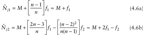
Burnham and Overton (1978) proposed the use of jackknife estimators up to the fifth order for estimating population size. Jackknife estimators were developed as a general technique to reduce the bias of a biased estimator. Here the biased estimator is the number of animals observed. The basic idea with the jth-order jackknife method is to consider subsets of the data by successively deleting j occasions from the original data. An appealing property of the jackknife approach is that the final estimates have closed forms. For example, the first-order and the second-order jackknife estimators turn out to be

Higher orders of the jackknife estimators are given in Otis et al. (1978, p. 109). Burnham and Overton (1978) also proposed a sequential testing procedure to select the best order. They recommended an interpolated jackknife estimator. All jackknife estimators are linear functions of capture frequencies and approximate variances can be derived.

Although Cormack (1989, p. 404) pointed out that there is no theoretical advantage to using this approach, the jackknife has performed well in simulations. Based on various simulation results, Otis et al. (1978, p. 34) commented that the jackknife estimator has a tolerable bias if the number of trapping occasions is sufficiently large (say greater than 5) and if a negligible number of animals are untrappable. As f₁ ≤ M_{k + 1}, it is seen from (4.1a) that the first-order jackknife estimate is always less than 2M_{k + 1}. Therefore, it usually underestimates the true population size when the mean capture probabilities are small, as shown in Chao (1988). On the other hand, if nearly all animals are captured, the jackknife methods tend to overestimate the population size. The jackknife methodology does not provide a measure to quantify the degree of heterogeneity among the animals.

Applying the jackknife technique to the data in table 2.1 by substituting M_{k + 1} = 38, k = 6, f₁ = 9, and f₂ = 6 into (4.1) gives = 45.5 (standard error 3.7) and = 48.3 (standard error 5.7). A sequential test applied to M_{k + 1} and successive orders of jackknife estimators results in an interpolated jackknife of 44.0 (standard error 4.0).

Since the proposal of the jackknife estimator, a number of researchers have presented various alternative approaches and compared their relative merits. The advances are quite substantial and some of them will be introduced later.

MODEL M_bh: P_ij = p_i UNTIL FIRST CAPTURE AND P_ij = c_i FOR ANY RECAPTURE

If model M_h is generalized to allow the individual capture probability to depend on previous capture history, it gives model M_bh. This model is equivalent to a heterogeneous removal model in which each animal is removed with a different probability. Thus, it also finds wide applications in removal and catch-effort studies, especially in fishery science.

Model M_bh has some of the disadvantages of models M_b and M_h. Like model M_b, only the first captures carry information about the population size. Like model M_h, the individual heterogeneity effects cause theoretical difficulties. For this model, Otis et al. (1978) proposed a generalized removal method. This is based on the idea that animals with larger removal probabilities tend to be removed in earlier occasions than animals with small removal probabilities. Conditional on those animals not previously removed, the average removal probabilities of the k occasions are expected to be decreasing. For a homogeneous population, these conditional removal probabilities are constant.

The generalized removal method first considers fitting a simple model with all average removal probabilities equal. If the simple model fits the data well, then the model is reduced to model M_b. In this case, the inferences are identical to those of model M_b. If this model does not fit, then consider a model where the removal probability on the first occasion is larger than the others. In other words, it is basically assumed that after u₁ animals have been removed, the remaining N − u₁ animals have identical probabilities of being removed and can be fitted to model M_b. The generalized removal method fits successively more general models until an acceptable fit is found. Then the population size is obtained based on the final selected model.

The reason for setting the average probabilities equal (except for the first few) is to reduce the number of parameters. However, it may contradict the finding of decreasing probabilities mentioned above. Under the model assumption, even if some animals with large removal probabilities are removed, heterogeneity still exists and model M_b is not theoretically valid for the remaining animals, especially when removal probabilities vary greatly. Simulation studies (Otis et al. 1978, p. 130; Pollock and Otto 1983, p. 1043) have shown that the generalized removal estimator typically has a negative bias, which can be large if the removal probabilities are very heterogeneous. An improved estimator due to Pollock and Otto (1983) is described below.

For the first-capture data (u₁, u₂, … , u₆) in table 2.2, the model assuming that all removal probabilities are equal fits well. The resulting estimate of the population size is 41.0 (standard error 3.1), which is the same as obtained with model M_b. The average removal probability is estimated to be 0.34, which is identical to the estimated first-capture probability in model M_b.

MODEL M_th: P_ij = p_ie_j

This model combines time and heterogeneity effects, with a multiplicative form of the effects being assumed. No estimator of population size had been suggested at the time that the paper by Otis et al. (1978) was published.

In some capture–recapture studies for large animals, actual recapture is not necessary and records of resighting suffice to provide the necessary recapture information. In this case, there is no need to model any behavioral response to capture. As a consequence, model M_th may be a reasonable model. It can also be considered when different trapping methods are feasible. In applications to human populations, usually different ascertainment methods (e.g., occurrence on different lists of patients) are used to “capture” individuals. Hence, this model is potentially useful in analyzing multiple-list problems. Recent developments of this model are considered below.

MODEL M_tbh: P_ij = p_ij UNTIL FIRST CAPTURE AND P_ij = c_ij FOR ANY RECAPTURE

In this model, three sources of variations in capture probabilities are considered. This most general model has previously been considered only conceptually useful and too complicated to be applied to practical situations if no restrictions are made. However, the general model M_tbh has been selected as the most likely model for estimating the size of squirrel (White et al. 1982, p. 149) and mouse (Otis et al. 1978, p. 93) populations. If reasonable assumptions can be made, then an estimation procedure for this model would offer a unified approach for all eight models. New methodologies that usually require extensive numerical computations have been developed and are discussed below.

New Approaches

In the past two decades, there has been an explosion of methodological research on capture–recapture. In the remainder of the chapter some of these methods are described and illustrated using the data of table 2.1.

BOOTSTRAP METHODS

For models without individual heterogeneity, standard likelihood theory yields a large-sample variance estimator for the MLE. Often this variance approximation may not be adequate for small samples. Moreover, for heterogeneous models, the corresponding likelihood functions are mathematically intractable. The use of resampling methods such as the bootstrap has been proposed (Efron and Tibshirani 1993; Buckland and Garthwaite 1991) to obtain variance estimators. The bootstrap is applicable to a variety of capture–recapture models (Chao et al. 2001b). The procedure is to resample capture–recapture data according to the relative frequencies of the observable capture patterns. Then a bootstrap estimate of population size is calculated using the resampled data. After many replications, the variance is estimated as the sample variance of all bootstrap estimates. Resampling techniques can also be used for obtaining confidence intervals.

IMPROVED INTERVAL ESTIMATION

The construction of traditional confidence intervals is based on the large-sample normality of population size estimators. Several drawbacks for this method have been noted (Chao 1987): (1) the sampling distribution is usually skewed; (2) the lower bound of the resulting interval may be less than the number of animals caught in the experiment; and (3) the coverage probabilities are often unsatisfactory. To overcome these problems, a log-transformation was suggested by Burnham and applied by Chao (1987). That is, the 95% confidence interval for any estimator with an estimated variance can be constructed as

where

The lower bound of this interval is always greater than the number of different animals actually captured in all occasions. Alternative approaches include the resampling methods mentioned above and the use of profile likelihoods (Cormack 1992).

MAXIMUM LIKELIHOOD ESTIMATOR FOR MODEL M_tb

Burnham derived the MLE of population size for model M_tb under the assumption that recapture probability, c_f, j = 2, . . ., k, is a power function of the initial capture probability, p_j; i.e., c_j = p_j^1/θ, for some parameter θ (Rexstad and Burnham 1991, p. 13). This MLE has been implemented in program CAPTURE. A parameter θ > 1 implies that the animals exhibit trap-happy behavior, while θ < 1 implies trap-shy behavior. Using CAPTURE, for the mouse data in table 2.1 = 40 (standard error 3.6), = 2.09, () = (0.37, 0.39, 0.26, 0.28, 0.43, 0.42), −2ln(L_tb) = 94.6 and AIC = 110.6.

A problem with this estimator is that the iterative steps may fail to converge even for nonsparse data. This motivated Chao et al. (2000) to find the MLE under the alternative assumption that the recapture probabilities bear a constant relationship to initial capture probabilities. That is, c_j / p_j = θ for all j = 2, … , k. The likelihood can be formulated (Chao et al. 2000) and an approximate variance derived. The case θ > 1 corresponds to trap-happy behavior and θ < 1 corresponds to trap-shy behavior. Using CARE-2 (a computer program introduced in section 4.4), and fitting the model to the data in table 2.1, gives = 2.34, () = (0.34, 0.33, 0.21, 0.23, 0.29, 0.27) and = 44.0 (standard error 6.9). Also, for this model, −2ln(L_tb) = 92.3 and AIC = 108.3.

The two versions of model M_tb applied to the mouse example show strong trap-happy behavior for the animals and slight time-varying effects. Each model is a significantly better fit to the data than model M_t (see section 1.4) but is not significantly different from model M_b. Thus, both versions of model M_tb and model M_b are appropriate for use in estimating population size. Model M_b is selected among the three adequate models because the AIC for this model is the lowest.

When time and behavioral response affect capture probabilities, the two approaches above provide applicable models. However, both models need sufficient capture information to allow for stable estimation, especially when there are many capture occasions.

JACKKNIFE TECHNIQUE FOR MODEL M_bh

When there are numerous parameters such as models M_h and M_bh, a non-parametric technique such as the jackknife has been used to construct new estimators. For model M_h, there is Burnham and Overton’s jackknife as given in equation 4.1. For model M_bh, Pollock and Otto (1983) recommended another type of jackknife, which was shown in simulations to be an improvement over the generalized removal estimator. This jackknife estimator has the simple form

It implies that the number of missing animals is estimated by (k − 1)u_k, depending only on the first captures caught on the last occasion. When nearly all animals are captured in the experiment so that several animals are newly caught on the last occasion, this estimator tends to overestimate. For the frequency data in table 2.2, the jackknife estimate is 53, which is much higher than the estimate from other models.

SAMPLE COVERAGE APPROACHES FOR MODELS M_h AND M_th

The sample coverage approach was originally applied to heterogeneous species abundance models (Chao and Lee 1992). Then Chao et al. (1992) and Lee and Chao (1994) modified it for application to capture–recapture experiments with emphasis on the models M_h and M_th. They assumed that the heterogeneity effects can be summarized in terms of the mean and coefficient of variation (CV) of p₁, p₂, … , p_N. This CV is a nonnegative parameter that characterizes the degree of heterogeneity. The CV is zero if and only if the animals are equally catchable, and the larger the CV, the greater the degree of heterogeneity among animals.

The sample coverage is defined as the proportion of the p_i’s that is associated with the individual variation among captured animals and it can be estimated in heterogeneous models. When there are at least five occasions, Chao et al. (1992) and Lee and Chao (1994) suggested the sample coverage estimator

and its bias-corrected form

Then the population size can be estimated via the estimation of sample coverage. The two population size estimators for model M_h are

where

is an estimator for CV². For model M_th, the estimators have similar form except for a different CV estimator (Lee and Chao 1994).

There are several advantages to the sample coverage approach: (1) it utilizes all the capture frequencies and has an explicit form; (2) a measure is provided to quantify the degree of heterogeneity; and (3) the estimator tends to the true population size when p₁, p₂, …, p_N are a random sample from a gamma distribution. The limitation is that a sufficient number of capture occasions (say, at least five) and sufficient capture information are needed to accurately estimate the CV parameter. The sample coverage approach applied to the data in table 2.1 yields, with model M_h, the two CV estimates and , which gives some evidence of heterogeneity. The two estimators in (4.4) are respectively (standard error 3.8) and (standard error 3.5). The results from model M_th, are not presented here, but were quite similar.

ESTIMATING EQUATIONS (INCLUDING MARTINGALE METHOD AND MAXIMUM QUASI-LIKELIHOOD)

Chao et al. (2001b) explored a general estimating equation and provided a unified approach for a special case of model M_tbh. The first-capture probability for the ith animal is designated P_ij = p_ie_j. This model combines the time effect for the jth occasion, e_j, and the heterogeneity effect for animal i, p_i, in a multiplicative form. Similarly, the recapture probability is C_ij = θp_ie_j (i.e., the recapture probability is proportional to the first-capture probability with the same constant of proportionality for all animals). To reduce the number of parameters and remove nonidentification, it was also assumed that the heterogeneity effects p₁, p₂, …, P_N are characterized by their mean and CV.

Although the likelihood is not generally obtainable, the moments (i.e., the expected values and variances of u_j and m_j) of first capture and recapture, for each capture occasion j, can be derived in terms of the mean and CV of the heterogeneity effects. Consequently, an estimating equation approach is available without much further restriction. This approach extends the martingale approach (Yip 1991; Lloyd 1994) and maximum quasi-likelihood method (Chao et al. 2000). This approach is computer intensive and a large number of capture and recapture data are needed to estimate time, heterogeneity, and behavioral effects. Otherwise, the iterations for estimation may not converge. As in all modeling, the more complex the models, the more data are required to obtain reliable parameter estimates.

When the estimating equation approach is applied to the data in table 2.1, the following population size estimates are obtained, along with estimated bootstrap standard errors for the heterogeneous models: model M_h: 40.0 (standard error 2.1); model M_th: 40 (standard error 2.2); model M_bh: 44 (standard error 4.4); model M_tbh: 44 (standard error 5.4). Unfortunately, the usual likelihood-based tests cannot differentiate between these models because the likelihood functions are not computable. See below for further discussion on model selection and model uncertainty.

It has been seen from fitting model M_b that the data show strong evidence of the trap-happy phenomenon. Recall that model M_b produces a population size estimate of 41.0 (standard error 3.1) with a 95% confidence interval from equation 4.2 of (39 to 53). In addition to the behavioral response, the further general models M_bh and M_tbh merit consideration. For this data set these models produce close results, so it is reasonable to adopt the most general model M_tbh and conclude that the population size is about 44 (standard error 5.4). The data based on model M_tbh show strong trap-happy behavior ( = 1.89), a low degree of heterogeneity (the CV estimate is 0.36), and slight time-varying effects as the relative time effects are estimated to be () = (0.34, 0.32, 0.26, 0.26, 0.33, 0.33), where denotes the average of p_i’s .

Usually, a simpler model has smaller variance, but larger bias, whereas a general model, because it includes more parameters, has lower bias but larger variance. The 95% confidence interval using (4.2) under model M_tbh, for example, is 40 to 65. An objective selection rule between models M_b and M_tbh is currently not available. A simpler model produces narrow confidence interval with possibly poor coverage probability, whereas a more general model produces wide interval with more satisfactory coverage probability. This trade-off is clear in comparisons of the different models built around our deer mouse data.

OTHER APPROACHES

Some other important methods will now be briefly considered. See the relevant references for details and software.

Log-linear or Generalized Linear Models

This approach models the observable frequency counts of unique capture histories as a log-linear model or a generalized linear model. Then a model is selected and used to estimate the missing cells. Model selection and model testing then can be performed under a unified framework (Fienberg 1972; Cormack 1989; Agresti 1994; Coull and Agresti 1999; Evans et al. 1994; IWGDMF 1995). The simplest independent log-linear model is equivalent to the classical model M_t discussed in chapter 2. Chao et al. (2001a) describes the relative merits of this approach.

Bayesian Methods

In the past, a limitation of classical Bayesian estimation approaches was the complex calculations involved. Now this problem can be overcome by the use of Gibbs sampling, a Monte Carlo Markov Chain technique (Castledine 1981; Smith 1988, 1991; George and Robert 1992; Lee and Chen 1998). With the Bayesian approach, empirical information can be incorporated and nonidentifiable models can also be treated (Lee and Chen 1998). However, there have been arguments about the sensitivity of the Bayesian estimates to the choice of priors (Chao 1989). Huggins (2002) has developed an empirical Bayes approach for model M_h assuming a beta distribution of the capture probabilities.

Parametric Approaches for Modeling Heterogeneity

Lloyd and Yip (1991), Sanathanan (1972), and Coull and Agresti (1999), respectively, used beta, gamma, and normal distributions to model heterogeneity. This approach reduces the number of parameters to only a few and thus traditional inference can be easily applied. A difficulty in this approach is that several models may adequately fit the data, but the estimated population sizes may differ greatly among models (Link 2003). It is important to remember that many difficulties can result from assuming a particular mathematical form for data without including an appropriate level of biological intuition to check whether the assumptions are compatible with common sense.

Latent Class, Mixture Model, and Nonparametric Maximum Likelihood

This approach assumes that the population can be partitioned into two or more homogeneous groups (Darroch et al. 1993; Agresti 1994; Norris and Pollock 1996b; Coull and Agresti 1999; Pledger 2000) so that a latent class or a finite mixture can be applied to model capture probability. Pledger (2000) found that for many data sets a simple dichotomy of animals is enough to correct for bias due to heterogeneity. See Link (2003) for relevant discussion.

Model Selection, Model Uncertainty, and Model Averaging

Model selection is an important topic in statistical inference (Buckland et al. 1997). Currently preferred model selection procedures using likelihood ratio tests or the AIC criterion (among models for which likelihoods are obtainable) were discussed in section 1.4. Stanley and Burnham (1998) commented that the existing model selection procedure in CAPTURE (Otis et al. 1978) usually selects an inappropriate model in simulations. For models with heterogeneity, the likelihoods are usually not computable unless parametric assumptions are made. Currently there is no objective method to select a model from the various heterogeneous models. Stanley and Burnham (1998) proposed the use of a model-averaging concept, in which weighted estimates from competing models are combined. Norris and Pollock (1996a) also considered model uncertainty in the estimation of variances.

Table 4.1 (Chao 2001) summarizes for each model the available approaches that are known. References are provided in the table for modeling approaches that have not been addressed in the above discussion.

We remark that capture–recapture models have wide applications to nonanimal populations in other disciplines. Some applications include the estimation of plant populations (Alexander et al. 1997), elusive human populations (e.g., cases for a specific diseases, homeless persons, and mentally ill people [IWDGMF 1995]), the size of vocabulary for an author in linguistics (Efron and Thisted 1976), the number of undetected bugs in a piece of software in software reliability (Briand et al. 2000), and the number of undiscovered genes in genetics (Huang and Weir 2001).

Models Incorporating Covariates

Individual, environmental, or other auxiliary or concomitant variables recorded or measured in capture–recapture experiments commonly are called covariates. Using such variables, sophisticated models may be fitted that both estimate the population size and give insight into the capture process (Huggins 1989, 1991; Alho 1990).

Pollock et al. (1984) proposed a model to incorporate covariates in the analysis. They developed an estimation procedure based on the full likelihood. However, the covariates for the uncaptured animals are not observable. Therefore, they had to categorize all animals into several groups and use the midpoint of the classifying covariate as a representative covariate for a group. Huggins (1989, 1991) avoided this difficulty by using a likelihood conditional on the captured animals, so that the covariates of uncaptured animals are not needed in the analysis.

TABLE 4.1
Discrete-time models and associated estimation methods

Model	Approaches/methods
Mtbh	Estimating equationa (Chao et al. 2001b) Generalized linear models using covariatesa,b (Huggins 1989, 1991) Conditional sample coverage (Lee 1996) MLE using mixture (Pledger 2000) (All approaches are valid for the submodels given below; some of them are not repeated in each model)
Mbh	Generalized removalc (Otis et al. 1978) Jackknifea,c (Pollock and Otto 1983) Sample coveragea (Lee and Chao 1994) Estimating equationa (Chao et al. 2001b) Nonparametric MLE (Norris and Pollock 1995, 1996b)
Mtb	MLEa,b,c (Rexstad and Burnham 1991; Chao et al. 2000) Estimating equation or martingale methoda (Lloyd 1994; Chao et al. 2001b) Bayes approach (Lee and Chen 1998) Log-linear models (Cormack 1989)
Mth	Sample coveragea,c (Lee and Chao 1994) Estimating equationa (Chao et al. 2001b) Mixed logit models (Agresti 1994; Coull and Agresti 1999) Log-linear models or latent class models (Darroch et al. 1993; Agresti 1994)
Mh	Jackknife methoda, c (Burnham and Overton 1978) Moment estimatorc (Chao 1987) Sample coveragea (Lee and Chao 1994) Estimating equationa (Chao et al. 2001b) Martingale method (Lloyd and Yip 1991) Bootstrap estimator (Smith and van Belle 1984) Empirical Bayes approach (Huggins 2002) Nonparametric MLE (Norris and Pollock 1995, 1996b)
Mb	MLEa, b, c (Zippin 1956) Estimating equation or martingale methoda (Lloyd 1994) Log-linear models (Cormack 1989)
Mt	MLEa, b, c (Darroch 1958; Otis et al. 1978) Moment estimatorc (Chao 1989) Estimating equation or martingale methoda (Yip 1991) Binomial model (Schnabel 1938) Log-linear models (Fienberg 1972) Bayes and empirical Bayes (Castledine 1981; Smith 1988, 1991; George and Robert 1992)
M0	MLEa, b, c (Otis et al. 1978) (All estimators given above are valid here)
a Available in software CARE-2. b Available in software MARK. c Available in software CAPTURE. Source. Chao (2001).

To illustrate the covariate analysis, note that there were actually three covariates—sex (male or female), age (young, semi-adult or adult), and weight—collected for each individual in the deer mouse data of table 2.1. The complete data are shown in table 4.2. Only three semi-adult mice were caught, so they were reclassified as adults. The variables sex and age are categorical and each has two categories. To include these covariates in the model, define the following dummy variables:

W_i1 = 1 if the ith animal is a male, and 0 for a female; and
W_i2 = 1 if the ith animal is a young, and 0 for an adult.

The covariate weight is a continuous variable, thus

W_i3 = weight of the ith animal.

Huggins (1989, 1991) proposed a logistic type of model for the first-capture probability of the ith animal on the jth occasion, P_ij, and also a similar form for the recapture probability C_ij as follows:

Here the parameter a denotes the intercept, a_j denotes the time-effect (with a_k = 0 because the last occasion is used as a basis for comparison), β₁ denotes the effect of being male, β₂ denotes the effect of being young, β₃ denotes the effect of a unit of weight, and υ denotes the effect of behavioral response. The above model is denoted by to distinguish it from the model without using covariates. Under this model, the individual heterogeneity is assumed to be fully determined by the observable covariates. The parameters β₁, β₂, β₃, a₁, a₂, … , a_k − 1, and υ denote, respectively, the heterogeneity, time effects, and behavioral response effect.

The interpretation of the coefficient of any β is based on the fact that when β > 0, the larger the covariate is, the larger the capture probability is, while if β < 0 then the larger the covariate is, the smaller the capture probability is. Also, the parameter υ represents the effect of a recapture, which implies that υ > 0 corresponds a case of trap happy and υ < 0 corresponds to the case of trap shy.

TABLE 4.2
Individual capture history of mouse with three covariates: sex (m: male, f: female), age (y: young, sa: semi-adult, a: adult), and weight (in grams)

It is sometimes more convenient to rewrite (4.5a) and (4.5b) as logit functions:

for the first-capture probability, and

for the recapture probability.

To construct the “conditional” likelihood proposed in Huggins (1989, 1991), consider, for example, the first mouse captured. Table 4.2 shows that this was a young male with weight 12, so that W₁₁ = 1, W₁₂ = 1, and W₁₃ = 12. With these covariates in equation 4.5, the probability for the first animal with capture history 111111 is P₁₁C₁₂C₁₃C₁₄C₁₅C₁₆. The idea here is that given the event that this mouse was captured, with probability

the likelihood is expressed as

Similarly, for the second young female mouse with weight 15 and history (100111), W₂₁ = 0, W₂₂ = 1, and W₂₃ = 15 and the conditional likelihood is

The full conditional likelihood is a product of 38 individual likelihoods and is a function of a, a₁, a₂, … , a₅, β₁, β₂, β₃, and υ. Therefore, numerical methods must be used for finding the (conditional) MLEs. After the MLEs of the parameters are obtained, the population size is estimated by the Horvitz-Thompson (1952) estimator,

TABLE 4.3
Estimation results for various models with covariates

where is the estimated capture probability evaluated at the conditional MLE. The variance of the resulting estimator can be estimated by an approximate variance formula derived in Huggins (1989, 1991).

The logit approach allows the use of standard linear models to model the capture probabilities and conditional versions of the likelihood ratio test and AIC to compare submodels. Submodels of the most general model corresponding to those of Otis et al. (1978) are

Table 4.3 shows the results for fitting these models to the deer mouse data, using the software CARE-2 (to be introduced in section 4.4).

For each model, the corresponding estimated population size and its standard error, twice the maximized log-likelihood, the number of parameters and the Akaike Information Criterion (AIC) are shown. From the values of AIC in table 4.3, model is selected for this data set. Based on the selected model, is the effect for a male (the female is set to be 0), so males have larger capture probabilities than females, and is the effect for a young (the adult effect is set to be 0), so young have larger capture probabilities than adults. The coefficient is the effect for a unit change of body weight. This implies the capture probability increases with the weight. Also , which provides evidence of trap-happy behavior. The estimated population size under the selected model is 47 (standard error 7.2), and a 95% confidence interval using (4.2) is 40 to 74. This logistic model simultaneously models a behavioral response and heterogeneity based on the observable covariates. Recall that if covariates are ignored, the estimating equation approach for both models M_bh and M_tbh yield an estimate of 44, and the latter provides a 95% confidence interval of 40 to 65.

Advantages for models incorporating covariates include the following: (1) the models provide a clear description of the sources of heterogeneity, and the effect of each covariate can be assessed; (2) model comparisons and model selection can be performed under a unified framework; and (3) if all relevant covariates are included, then these models generally yield better estimators with respect to bias and precision, though the above analysis of the mouse data could not show this. One assumption is that the heterogeneity effects are fully determined by the observable covariates. The use of covariates does not take into account the heterogeneity due to unobservable innate characteristics of the individuals. If some important covariates were not recorded, the models might work less well than those without using covariates.

4.3 Continuous-time Models

For insects or large mammals, trapping is often conducted over a fixed period of time, and captures (or sightings) of individuals can occur at any time during the data collection. Thus, there is only one capture on each capture occasion (i.e., sample size of 1) and the exact time for each capture is recorded. This type of experiment is referred to as a continuous-time capture–recapture experiment.

Data Structure

An early paper by Craig (1953) described a continuous-time experiment, in which one butterfly was netted at a time, marked with a spot of nail polish, and then released immediately. Darroch (1958) discussed the analysis for samples of size 1, though these authors did not refer to their methods as continuous-time models. In most large-mammal studies, usually only one individual can be captured or sighted at a time. Actual capture or marking is not always necessary because large animals can sometimes be uniquely identified by physical characteristics, such as shape, scars, color variation in fur, geographically separated territories, etc. This type of continuous-time model is therefore particularly useful for studies based on sightings or photographs of animals such as whales (Whitehead and Arnbom 1987) and bears (Mace et al. 1994; Boyce et al. 2001; Keating et al. 2002). Some of the bear-sighting data sets of Boyce et al. (2001) and Keating et al. (2002) are used for an example.

TABLE 4.4
Hypothetical example of continuous-time data

The model being considered is also a general framework for species richness estimation where a “unique individual” is equivalent to a species and a “capture” means that a species is represented in a sample. A pioneering paper in this area is by Fisher et al. (1943). A review is provided by Bunge and Fitzpatrick (1993), and Chao (2005) and Wilson and Anderson (1995) and Wilson and Collins (1993) provided some simulation comparisons of estimation methods.

For each captured animal the complete history consists of a series of exact capture times. A small hypothetical example will be used to explain the data structure. Assume that there are 6 animals in a population (N = 6) and four animals are caught in a total of 9 captures in the time period of (0, T). The capture times for the four animals and the capture frequencies shown in table 4.4.

For the models to be discussed below, the statistics needed for estimation are the frequency counts f₁, f₂,…, f_s, or functions of these counts, where s denotes the maximum frequency and f_j denotes the number of individuals that are captured exactly j times in the time interval (0, T). The complete capture information for the above data can therefore be summarized as follows, where M denotes the number of distinct animals caught and n the total number of captures:

Out of 9 captures, 4 distinct individuals were captured; two of them were captured once, one was captured three times, and one was captured four times. It is clear that f₁ + f₂ + … + f_s = M and f₁ + 2f₂ + … + sf_s = n.

The Classical Homogenous Model

Assume that the capture or sighting process is a Poisson process with rate parameter λ in the time period of (0, T). This means that the probability of capturing an animal in a small interval around t, say (t, t + dt), is approximately λdt, and the captures in two nonoverlapping intervals are independent. The number of captures in any time interval (t₁, t₂) is a Poisson random variable with parameter λ(t₂ − t₁), which implies that the probability of no capture in this interval is exp[−λ(t₂ − t₁)].

With the classical homogeneous model the Poisson rate parameters for all animals are identical and constant over time. This model is a continuous-time version of model M₀. The intuitive approach of Crowder et al. (1991, p. 165) can be used to obtain the likelihood. For the first captured animal in the example, consider the following consecutive events in nonoverlapping intervals: no capture in (0, 1.6), one capture in (1.6, 1.6 + dt₁), no capture in (1.6 + dt₁, 4.0), one capture in (4.0, 4.0 + dt₂), no capture in (4.0 + dt₂, 5.3), one capture in (5.3, 5.3 + dt₃), and no capture in (5.3 + dt₃, T). Then the joint probability of these events is equal to the product of the probabilities as given by

Dividing the above product probability by dt₁dt₂dt₃ and letting dt₁, dt₂, dt₃ all tend to zero gives the likelihood for the first animal as λ³ exp(−Tλ). It is clear that only the capture frequency is relevant in the estimation procedure. Similarly, the likelihoods for the second and the third animals are, respectively, – exp(λTλ) and λ²exp(−Tλ). For the animals that are not captured, the probability is exp(−Tλ). Moreover, in a homogeneous model, the number of possible divisions of 6 individuals into 5 frequency groups with frequencies 0, 1, 2, 3, 4 and sizes 2, 2, 0, 1, 1 is 6!/(2! 2! 0! 1! 1!). As a result, the full likelihood for the data is

Generally, under a homogeneous model, the full likelihood becomes

In this special homogenous case, the statistics M and n are sufficient for estimating the parameters N and λ and the MLE can thus be obtained by maximizing the above likelihood. It follows from Craig (1953, p. 172) that the exact MLE of N is the solution of the following equation:

Darroch (1958, p. 349) obtained an approximate MLE as the solution of the equation

An approximate variance estimator can be obtained by substituting an estimate of N into the variance formula

Becker (1984) and Becker and Heyde (1990) extended the above model to the case where the Poisson rate is a time-varying function, λ(t) in the interval (0, T), i.e., for the continuous-time version of model M_t. These authors found that the estimation procedures are identical to those for model M₀.

Heterogeneous Models Using Bear-resighting Data

The homogeneity assumption is questionable in most applications. A heterogeneous model M_h can therefore be considered. In this model, capture rates are allowed to vary among individuals by assuming that the capture process for the ith animal is a Poisson process with rate λ_i. As in discrete-time models, assumptions are needed to model the parameters λ₁, λ₂, … , λ_N. Parametric approaches have been adopted by assuming that λ₁, λ₂, … , λ_N are selected from a distribution. A common choice is the gamma distribution, which was proposed by Greenwood and Yule (1920) and Fisher et al. (1943). Tanton (1965) and many subsequent authors have applied it to wildlife studies, including recent applications to bears (Boyce et al. 2001; Keating et al. 2002). The model is referred to as a Poisson-gamma model or a negative binomial model because the capture frequencies follow a negative binomial distribution. See Chao and Bunge (2002) for details of the likelihood and the estimation procedures. Other possible parametric family includes the log-normal (Bulmer 1974) and the inverse Gaussian (Ord and Whit-more 1986).

The continuous-time model can be regarded as a special case of the discrete-time model with all sample sizes being one. The jackknife and sample coverage approaches discussed in discrete-time model M_h can be applied directly here by replacing M_{k + 1} and k by M and n. That is, the first-order and the second-order jackknife estimators in equation 4.1 now become

TABLE 4.5
Sighting frequencies of female grizzly bears

From equation 4.4, a similar sample coverage approach (Chao and Lee 1993) results in the following estimators:

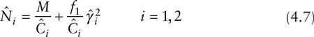
where the two coverage estimators are the same as before, but the estimator of the CV of λ₁, λ₂, … , and λ_N is slightly different. Here there is the following estimator for CV²:

If the sample size n is large, the two sample coverage estimates (Ĉ₁ and Ĉ₂), and thus the two population size estimates (), differ little in continuous-time models. In species number estimation some species may be very abundant, which leads to a large value for the CV. In that case, a bias-corrected estimator of the CV is needed and given in Chao and Lee (1992).

Boyce et al. (2001) and Keating et al. (2002) recorded the sighting frequencies of female grizzly bears with cubs-of-the-year in the Yellowstone ecosystem. The data for 1996–98 are used here for an example (table 4.5).

Boyce et al. (2001) considered the joint estimation of population sizes over years and assumed that the shape parameter of the gamma distribution was constant over time. Their estimates are shown in table 4.6. Keating et al. (2002) adopted a sample coverage approach and the estimate based on equation 4.7 is shown for each year. The table also shows the estimates under a homogenous model (i.e., model M₀), two jackknife estimates, and the estimate obtained from a Poisson-gamma model. A disadvantage for the Poisson-gamma approach is that in some cases (e.g., for 1996) the iterative steps for MLE do not converge.

TABLE 4.6
Estimates (with standard errors) for bear-sighting data

For the data of 1996, the estimated CV is = 0. This indicates equal sightability and it is reasonable to assume a homogeneous model. The sample coverage approach yields a very close result to that for a homogenous model. For the years of 1997 and 1998, the CV estimates are, respectively, = 0.57 and 0.45, which provide evidence of heterogeneity. Thus, the results under a homogeneous model would underestimate the true population size. The estimates are very close to those for , so they are omitted in table 4.6. The first-order jackknife and the sample coverage approach show that the numbers of female bears was stable over the three years.

General Models and Assumptions

As in the discrete-time models, a series of eight continuous-time models can be postulated depending on the sources of variability in the Poisson rates due to time, behavioral response, and heterogeneity. Consider a Poisson process with parameter (t), which can be intuitively interpreted as capturing animal i in a small time interval around time t. The Poisson rate for model M_tbh is given by

Here α(t), {λ₁, λ₂, … , λ_N}, and ϕ represent the effects of time, heterogeneity, and behavioral response, and α(t) is any arbitrary time-varying function in (0, T). All submodels can be formulated as shown below. Compared with discrete-time models, there has been relatively little published research for the continuous-time counterparts. Relevant references are given for each model:

Beyond the classical MLE approach, Becker (1984) was the first to establish a counting process framework for model M_t. Most subsequent authors dealing with the other models have followed this approach. Until now, there have been no estimation methods proposed in the literature for the most general model M_tbh and model M_bh. However, if the heterogeneity effects can be fully explained by observable covariates, Lin and Yip (1999) and Hwang and Chao (2002) explored a unified likelihood-based approach.

The data collected in continuous-time format provide more information than those in discrete-time models because the latter ignores recaptures of the same animals in any fixed occasion. In practice, more effort is usually needed to record the capture time for each captured animal. If times are not recorded, that information is lost to future analysis attempts. There has been little published work for comparing the relative merit of continuous-time models and their corresponding discrete-time models. We have found that estimates derived from continuous-time experiments will generally be more precise than those from discrete-time experiments, all other considerations being equal. It is not difficult to show that under a classical homogeneous model that the asymptotic variance of the MLE for population size under a continuous-time model is less than that under its corresponding discrete-time model. A similar conclusion is expected for other models. The gain in precision usually is most significant when only a small fraction of animals is captured in the experiment. Then, continuous-time models are clearly preferable to their corresponding discrete-time models. In contrast, if a relatively large number of animals is captured, estimators under the two types of models perform similarly (Wilson and Anderson 1995). In this case, there is almost no difference between the two types of models.

Relationship to Recurrent Event Analysis

In many studies, individuals may experience repeated events and times of each event are recorded. For example, in industrial reliability, repeated events include failures or repairs of a system (Lawless and Thiagarajah 1996). In medical studies, repeated events include recurrences of tumors, infections, and other diseases. There is a large literature on models for the recurrent event analysis (Wei and Glidden 1997). Most of the analyses have adopted Cox’s proportional hazard models based on a counting process approach (Andersen et al. 1993).

If each capture is regarded as a recurrent event then the continuous-time model can be treated as a special case of recurrent event analysis. Using this concept, the models presented above can be connected to recurrent event analysis. Many models using successive or cumulative capture times in recurrent event analysis can then be applied to capture–recapture models. However, there is a difference between the two approaches. In a recurrent event analysis, the number of individuals is usually known and the main parameter of interest is the effect of each covariate, whereas in a capture–recapture study the population size is the parameter of main interest. In a sense, these modeling approaches could be viewed as flip sides of each other. Clearly, the interaction of the two topics is a fruitful area for future research.

4.4 Computing Considerations

Information on the specialized computer programs needed for estimation for closed populations is provided in chapter 10 of this book. An additional program is necessary to accommodate recently developed estimators and the covariate methods initiated by Huggins (1989, 1991). A program CARE (for capture–recapture) containing three parts (CARE-1, CARE-2, and CARE-3) has been developed and is available at the website chao.stat .nthu.edu.tw. CARE-1 is an interactive S-PLUS program for the analysis of multiple lists (Chao et al. 2001a). CARE-2, a Windows 98 (or later) executable program written in the C language, calculates various estimates for the models with and without covariates that are described in section 4.2, as shown in table 4.1. The third part of CARE, CARE-3, written in GAUSS language, is an integrated program for analyzing the class of continuous-time models presented in section 4.3. A brief user guide with examples is also provided at chao.stat.nthu.edu.tw.

Figure 4.2. Flipper-tagged female Californian sea lion (Zalophus californianus) with her pup at Piedras Blancas, California in 1995. (Photo by Steven C. Amstrup.)

Since some special continuous-time models presented in Section 4.3 are equivalent to species estimation problems, a relevant computing program for the latter is EstimateS (Colwell 1997), which calculates various estimates of species richness including the jackknife and the sample coverage approach. The program is available from the website viceroy.eeb .uconn.edu/estimates.

4.5 Chapter Summary

• Discrete-time capture models are described. Discrete-time models assume that several trapping occasions have occurred, and that a group of animals is caught on each occasion such that the capture time of individuals within the occasion is not known.

• The eight models of Otis et al. are described as a basis for estimating population sizes, where these allow capture probabilities to vary with one or more of the factors of time, a behavioral response to capture, and individual variation in capture probabilities. Methods of estimation are discussed for each of the models.

• Newer approaches to estimation are discussed involving bootstrapping, improved confidence interval methods, parametric maximum likelihood estimation, jackknifing, sample coverage methods, estimating equation methods, generalized linear models, Bayesian methods, parametric modeling of heterogeneity distributions, latent class models, mixture models, and nonparametric maximum likelihood.

• Model selection and related problems are discussed briefly.

• The use of models involving covariates is reviewed, including those that assume logistic regression types of functions. It is shown how this approach can be used with each of the eight models of Otis et al.

• Continuous-time models are described for situations where the capture time is known for each captured animal. For this situation the classical homogenous model is described, where captures follow a Poisson process with a constant rate parameter. Heterogeneous models (parametric and nonparametric) are then considered, where the probability of capture varies from animal to animal.

• The relationship of continuous-time models to recurrent event analysis is noted.

• Computer programs for estimation are briefly discussed.